Resources
Dynamic Programming
Dynamic Programming (DP) is an optimization approach for solving complex problems by decomposing them into a sequence of simpler sub-problems (stages). Unlike Linear Programming, there is no single universal algorithm; rather, DP requires modeling problems based on specific principles and recursive relationships.
Bellman's Principle of Optimality
An optimal policy has the property that, regardless of the initial state and decision, the remaining decisions must constitute an optimal policy with regard to the state resulting from the first decision. This principle allows us to break down problems into stages and solve them recursively.
Modelling
Dynamic Programming problems are typically modeled using a state space representation, containing stages with states and decisions that transition between states. The key components include:
Stages & States
Stages represent the sequential steps of the problem, often corresponding to time periods or decision points. A model has stages with index . Each stage has a set of states containing all possible states at that stage.

Here, and with , meaning the algorithm is in node 11 at stage 2.
Decisions & Transitions
At each stage, a decision is made that influences the transition to the next state; the transition is noted as . The decision space defines the feasible decisions for each state at stage. The transition function determines how the current state and decision lead to the next state:
- State Transition Function: defines how the current state and decision lead to the next state.
- State-Dependent Cost Function: represents the cost incurred at stage when in state .
- Backward Recursive Cost Function: is the total cost from state in stage to the final stage if decision is made.
- Minimum Total Cost Function: is the minimum total cost from state in stage to the final stage, considering all feasible decisions.
Algorithms
| Feature | Backward Recursion | Forward Recursion |
|---|---|---|
| Direction | Starts at stage (end) and moves to (start). | Starts at stage (start) and moves to (end). |
| Initial State | Unknown or flexible (we find the best starting decision last). | Fixed (e.g., 0 investment, start node). |
| End State | Fixed (e.g., destination node, 0 inventory). | Unknown or flexible (e.g., any budget usage limit). |
| Use Case | Routing problems (Commuter), Inventory/Ordering problems. | Allocation problems (Capital Budgeting), Knapsack-style problems. |
| Equation |
Backward Recursion
Backward recursion starts at the destination (stage ) with a known cost (usually 0 or salvage value) and works backwards to the starting stage . It’s the default approach for solving DP problems, and best for problems where the initial state is fixed but the path is unknown.
For each stage, the cost to reach the destination is calculated based on the costs of the next stage:
Forward Recursion
Forward recursion starts at the initial state and calculates cost accumulating towards . It’s best for problems where the end state is flexible.
For each stage, the cost to reach the destination is calculated based on the costs of the previous stage:
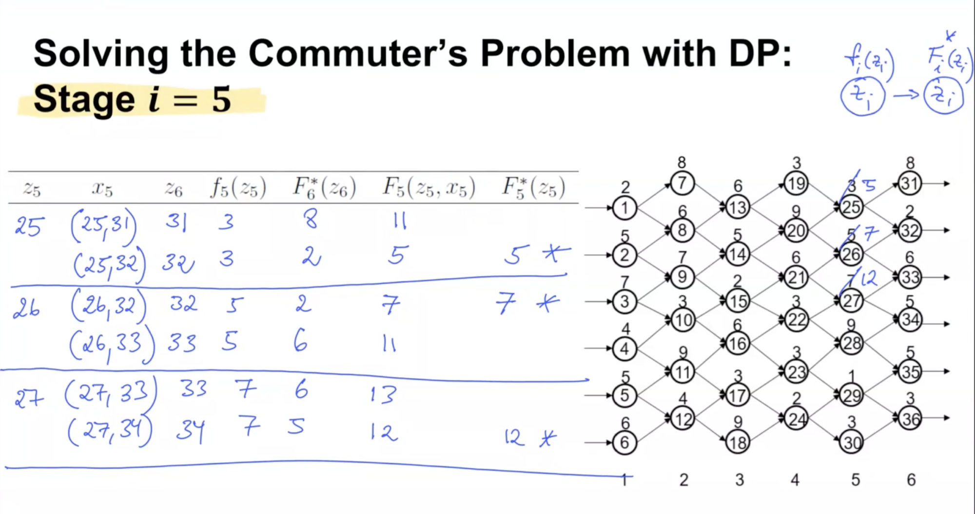
F^*_{i+1}(z_{i+1}) = \min_{x_i \in X_i(z_i)} \{f_i(z_i) + F^*_i(z_i)\}$$ # Applications: Problem Archetypes | Problem Archetype | Recursion Direction | Context & Source | | :------------------------------- | :------------------ | :------------------------------------------------------------------------------------------------------------------------------------------------------------------- | | **Commuter's Problem** (Routing) | **Backward** | The algorithm initializes costs at the final stage ($i=6$) and calculates the "Minimum Total Cost Function" backwards to the start ($i=1$). | | **Dynamic Ordering** (Inventory) | **Backward** | The slides explicitly define a "Backward Recursive Function" that calculates the cost from the current state to the final stage. | | **Capital Budgeting** (Knapsack) | **Forward** | The slides use a "Forward Recursion Function" where the state $Z_i$ represents the *total investments made after decision in stage i* (accumulating from the start). | | **Resource Allocation** (Sales) | **Backward** | The example demonstrates a "Backward Recursion Function," starting the calculation from the last sub-market ($i=3$) and moving to the first ($i=0$). | ## Deterministic Routing: Graph Traversal > [!info] Shortest Path Problem > > [[Network FIow Problems#dijkstras-algorithm|Dijkstra's algorithm]] is an application of DP to solve the shortest path problem, where the graph has non-negative weights on edges (representing travel times or distances). However, general DP can be applied to solve the shortest path problem even when negative weights are present, as long as there are no negative cycles. The algorithm iteratively computes the minimum cost to reach each node from the destination, allowing for the presence of negative weights. > [!info] Commuter's Problem > > The goal is to find the optimal route from a starting point to a destination, minimizing waiting time. > > - **Stages ($n$):** Each stage represents a column of intersections (e.g., $i=1 \dots 6$). > - **State ($z_i$):** The current intersection (node) the commuter is at in stage $i$. > - **Decision ($x_i$):** The next intersection (node) to move to in stage $i+1$. > - **Cost Function ($f_i(z_i)$):** The waiting time incurred at the current intersection $z_i$. > - **Recursion:** **Backward**. We calculate the minimum waiting time from the current intersection to the destination. > > ![[Pasted image 20260212154119.png]] > (circled number is node index, number above is waiting time) ## Dynamic Ordering: Inventory & Flow > [!info] Dynamic Ordering Problem > > The problem of determining the optimal inventory ordering policy over a finite time horizon to minimize costs. > > - **Stages ($n$):** Time periods (e.g., $i=1 \dots 5$). > - **State ($z_i$):** The inventory level at the **end** of period $i$ ($z_0=0$ and $z_n=0$). > - **Decision ($x_i$):** The quantity ordered (and delivered) at the **beginning** of period $i$. > - **Cost Function ($f_i(x_i, z_i)$):** Fixed ordering cost ($250$ if $x_i > 0$) + Variable holding cost ($1 \cdot z_i$). > - **Recursion:** **Backward**. We determine the minimum cost to satisfy demand from period $i$ to the end of the horizon. > > ![[Pasted image 20260212161154.png]] > Exemplary result on slide 40. > [!info] Ordering Policies > > - **Single Order in Period 1**: Order all inventory in the first period, which may lead to high holding costs. > - **Just in Time**: Order inventory in each period just before it is needed, minimizing holding costs but potentially increasing ordering costs. > > **An optimal order** only takes place if the inventory at the end of the previous period is 0 and equals the demand for the current period and optionally following periods: > - **Zero Inventory Ordering**: An order for period $i$ only takes place if the inventory at the end of period $i-1$ is 0. > - **Exact Requirements**: If an order $x_i > 0$ is placed in period $i$, the quantity must exactly equal the cumulative demand of periods $i$ through some future period $\tau$ (where $\tau = i, ..., n$). You never order a partial amount of a future period's demand. ## Resource Allocation: Knapsack **Capital Budgeting Problems**: The problem of allocating a limited budget across multiple investment projects to maximize returns is modeled using **Forward Recursion**. - **Stages ($n$):** Each project represents a stage. - **Decision ($x_i$):** $x_i = 1$ if project $i$ is selected, 0 otherwise. - **State ($z_i$):** The total capital invested after the decision in stage $i$ (accumulated from stages $1$ to $i$). - **Recursion:** We calculate the maximum value accumulating from the first project to the last. The transition function adds the cost of the current project to the previous accumulated investment state. > [!info] Sales Workers Allocation Problem > > The problem of allocating sales workers to different regions is modeled to maximize the total probability of success. > > - **Goal:** Maximize the total probability of success, which is calculated as the **product** of the probabilities of success of all sub-markets (not the sum). > - **Stages:** Each stage represents a sub-market. > - **State ($z_i$):** The number of salespersons available for markets 0 to $i$. > - **Decision ($x_i$):** The number of salespersons allocated specifically to market $i$. > - **Cost Function ($f_i(x_i,z_i)$):** The probability of success for market $i$ given the allocation of salespersons. > - **Recursion:** We determine the optimal allocation of the total workforce (e.g., 5 workers) across the three sub-markets to maximize the combined probability product. > > *This is very different from the traveling salesman problem.* > ![[Pasted image 20260212155234.png]]