Linear Programming

Resources

• Slides

Context

Relation to Economics

Linear Programming is the same as Linear Optimization. A mathematical model to achieve the best outcome in a system with requirements and an objective. The Lagragnian Method in Principles of Economics is used to solve constrained optimization problems.

In the context of Choosing an Approach, Linear Programming is used for simple decision making:

• Decision under certainty: Deterministic future within the modelled system
• Single goal
• Risk-neutral decision maker
• Static decision context

Phases of Operations Research Application

Problem → Modelling → Solving → Sensitivity Analysis → Decision Making

State of Tableau	RHS (Constants)	Objective Row Coefficients	Algorithm to Use
Feasible, Not Optimal	All $\ge 0$	At least one positive ($>0$)	Simplex
Infeasible, Optimal	At least one negative ($<0$)	All non-positive ($\le 0$)	Dual Simplex
Infeasible, Not Optimal	At least one negative ($<0$)	At least one positive ($>0$)	/ Big-M
Feasible, Optimal	All $\ge 0$	All non-positive ($\le 0$)	Done

Linear Programming Model

Linear Program

A mathematical model consisting of:

• Decision Variables: $x_1,x_2,...,x_n$
• Objective Function: linear function to maximize or minimize
• Constraints: linear equations or inequalities
• Non-negativity Restrictions: $x_i\ge 0$

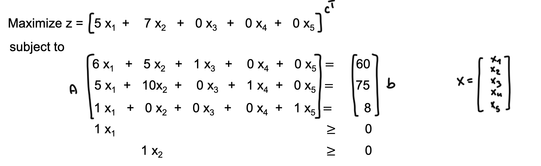
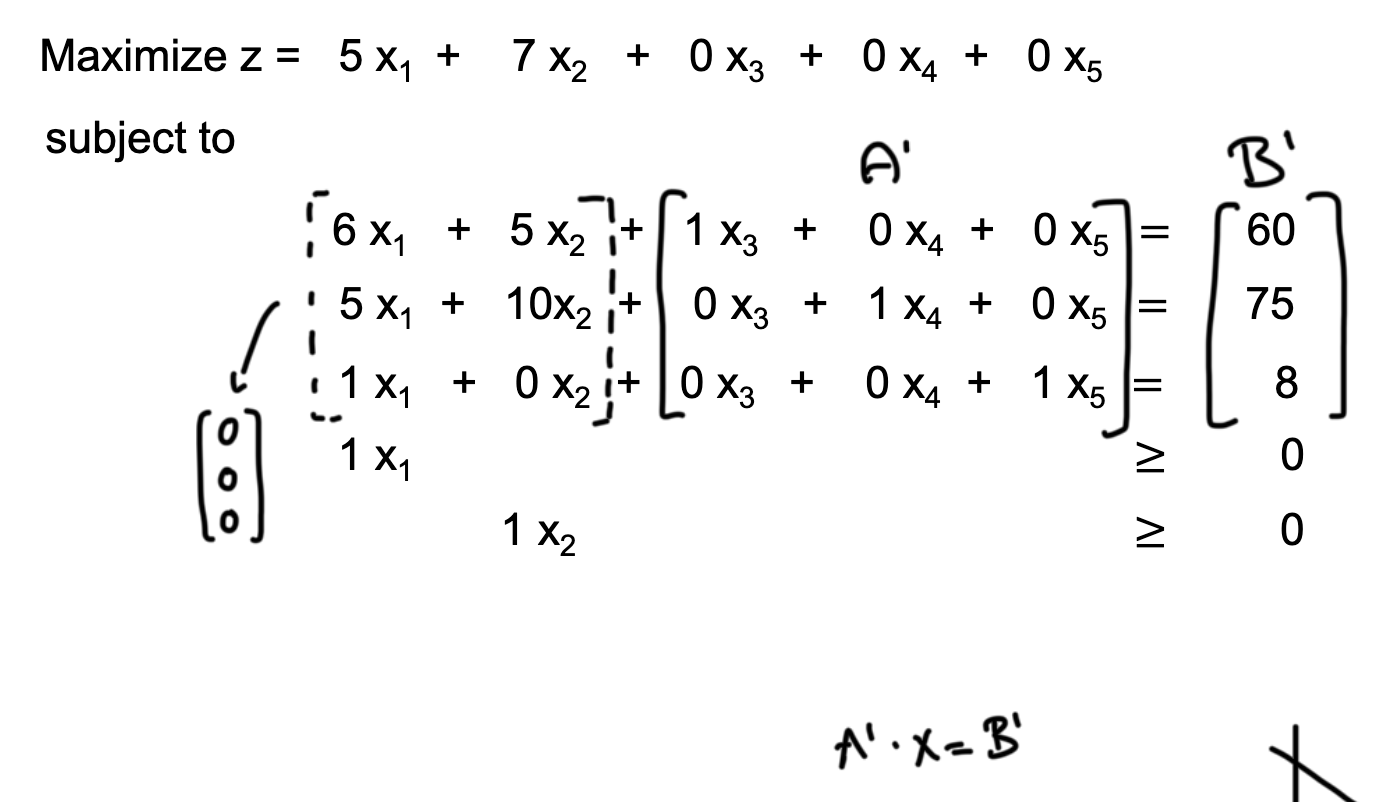
Matrix Form

• Objective Function: $maxz=c^{T}x$
• Constraints: $Ax\le b$, $x\ge 0$
• Where:
  • $z$: objective value
  • $c$: coefficients of the objective function
  • $x$: vector of decision variables
  • $A$: matrix of coefficients for constraints
  • $b$: vector of right-hand side values for constraints

Standard Form

The standard form, also called canonical form, is a specific representation of a linear programming problem that simplifies the application of solution methods like the Simplex algorithm.

Standard Form Requirements

• All variables are non-negative: $x_i\ge 0$
• All constraints are equalities: $Ax=b$
• The right-hand side values are non-negative: $b_i\ge 0$
• For each constraint, if it is a ‘less than or equal to’ (≤) inequality, a slack variable is added; if it is a ‘greater than or equal to’ (≥) inequality, a surplus variable is subtracted.
• The objective function is in maximization form.

If the right-hand side of a constraint is negative, the entire constraint is multiplied by $-1$.

Decision, Slack, Surplus, and Artificial Variables

• Decision Variables: Original variables representing choices.
• Slack Variables: Added to ‘less than or equal to’ (≤) constraints to convert them into equalities. They represent unused resources.
• Surplus Variables: Subtracted from ‘greater than or equal to’ (≥) constraints to convert them into equalities. They represent excess resources.
• Artificial Variables: Added to constraints that do not have an obvious initial basic feasible solution, meaning (0,0) is illegal due to $\ge$ or $=$ constraints. These are temporary variables used to facilitate finding an initial feasible solution.

Standardizing

To convert a linear program into standard form, first ensure the objective is maximizing, otherwise, multiply it by $-1$. Also ensure that restricted variables are non-negative (see below for unrestricted).

Then, to ensure that all constraints are equalities:

• For $\le$ constraints, add a slack variable $s_i\ge 0$: ${\sum }_{j=1}^n{a}_{i,j}\ast x_j+s_i=b_i$
• For $\ge$ constraints, subtract a surplus variable $s_i\ge 0$: ${\sum }_{j=1}^n{a}_{i,j}\ast x_j-s_i=b_i$
• If a constraint has a negative right-hand side, multiply the entire constraint by $-1$.

Unbounded variables are replaced by the difference of two non-negative variables:

• $x-\Delta L=50$ becomes $x-L^{+}+L^{-}$, with $L^{+},L^{-}\ge 0$.

Unrestricted Variables

Variables that can take any real value, positive or negative. To convert an unrestricted variable $x$ into non-negative variables, express it as the difference of two non-negative variables: $x=x^{+}-x^{-}$, where $x^{+},x^{-}\ge 0$.

Tableau Notation for Simplex

The tableau notation is used to keep track of coefficients, variables, constraints, and the objective function, in the standard approach of the Simplex Algorithm.

It has rows for each basic variable and the objective function, with columns for the right-hand side value and all coefficients (decision, slack, surplus, artificial).

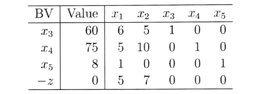
To quickly identify the next pivot point for Simplex, simply look for the largest positive coefficient in the objective function row (entering variable, here $x_2$) and the smallest positive ratio of right-hand side to column coefficient (leaving variable, here $x_4$).

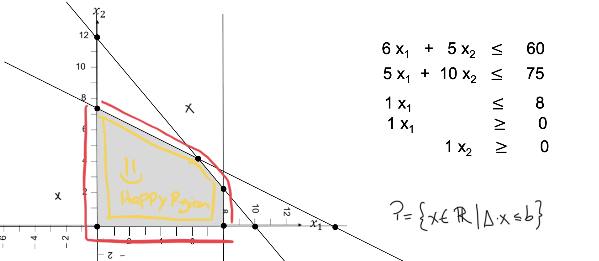
Graphical Representation

This is useful for programs with 2 decision variables, possible for 3, but not more.

The feasible region is the set of all points that satisfy the constraints, typically visualized in a 2D or 3D space. The feasible region polyhedron is formed by the constraint halfspaces intersecting.

The constraint function in an n-dimensional space: ${\sum }_{j=1}^n{a}_y\ast x_y=b$
For example, for $n=2$, this is a line: $a_1\ast x_1+a_2\ast x_2=b$

Extreme Points

The optimal solution lies at one of the vertices (extreme points) of the feasible region.

Extreme Point Definition

Given a polyhedron $P\in {\mathbb{R}}^n$, a point $x\in P$ is an extreme point if there are no two distinct points $y,z\in P$ such that $x=\lambda y+(1-\lambda )z$ for some $\lambda \in (0,1)$.

• The vertices of the feasible region can be found by solving the system of equations formed by the intersection of the constraint lines: $Ax=b$ (Slide 24).
• For a linear program with $n$ variables, defined by $m$ constraints/restrictions ($n\le m$), the number of possible extreme points is given by the binomial coefficient: $\left(\genfrac{}{}{0ex}{}{m}{n}\right)=\frac{m!}{n!(m-n)!}$ (Slide 25).
• Feasible: An extreme point that satisfies all constraints.

These extreme points are candidates for the optimal solution. Their feasibility and objective function value are evaluated (via software) to determine the best solution.

Simplex Algorithm

The Simplex Algorithm is an iterative method for solving linear programming problems in standard form. It finds the program’s optimal solution (or an unbounded solution) by moving from one vertex to another along the edges of the polyhedron defined by the constraints.

Prerequisite: LP in standard form with maximizing objective. The process also works with minimizing problems by inverting the selection criteria, but the course only covers maximization.

Basic and Non-Basic Variables

• Basic Variables: Variables that are part of the current solution basis, typically equal to the number of constraints.
• Non-Basic Variables: Variables that are not part of the current solution basis and are set to zero in the basic feasible solution.

In contrast to decision, slack, surplus, and artificial variables, basic and non-basic variables refer to the status of variables in the context of a specific solution.

Neighbor Basis

A neighboring basis is obtained by exchanging one basic variable with one non-basic variable. This exchange corresponds to moving from one vertex of the feasible region to an adjacent vertex along an edge.

Approach

$n$: number of variables; $m$: number of constraints; $j$: variable index; $i$: constraint index; ${\overline{c}}_j$: objective function coefficient of the current tableau; ${\overline{a}}_{i,s}$ coefficient of element $(i,s)$ in the current tableau; $b_i$: right-hand side value of constraint $i$ in the current tableau.

1. While there is at least one ${\overline{c}}_j>0$, repeat the steps below.
If $\overline{c_j}\le 0$, this is the optimal solution. If there is at least one positive coefficient in the objective function row, the current solution is not optimal. The solution is feasible as long as all basic variables are $\ge 0$.

2. Entering Variable: Choose a pivot column $s$ by selecting the variable with the largest positive coefficient in the objective function (the steepest ascent). This method is called Dantzig’s pivot rule.
${\overline{c}}_s=ma{x}_{j=1}^n\{{\overline{c}}_j\stackrel{ˉ}{}|{\overline{c}}_j>0\}$
If there is no such $s$ (no negative coefficient), the current solution is optimal.

Unbounded Solution

If all coefficients in the selected variable’s column are $\le 0$, the solution is unbounded in this direction. This is because if the objective coefficient is positive but all constraint coefficients are non-positive, increasing this variable will indefinitely increase the objective function without violating any constraints.

3. Leaving Variable: Choose a pivot row $r$ by selecting the smallest positive ratio of $\frac{b_i\text{(right side)}}{{\overline{a}}_{i,s}\text{(column coefficient)}}$, ignoring column coefficients $\le 0$. This represents the maximum amount the entering variable can increase before that constraint is violated.
$\frac{{\overline{b}}_r}{{\overline{a}}_{r,s}}=mi{n}_{i=1}^m\{\frac{{\overline{b}}_i}{{\overline{a}}_{i,s}}|{\overline{a}}_{i,s}>0\}$

4. Change basic variables, re-establish canonical form.
Include the new basic variable $x_s$ and exclude the old basic variable $x_r$ by pivoting (Gaussian Elimination). The pivot element should be $1$, while all other elements in the pivot column should be $0$.

To achieve this, the following row operations are performed:

• Divide the pivot row $r$ by the pivot element ${\overline{a}}_{r,s}$ to make the pivot element equal to $1$.
• For each other row $i$ (including the objective function row), subtract ${\overline{a}}_{i,s}$ times the new pivot row from row $i$ to make all other elements in the pivot column equal to $0$.
  Slack, surplus, and artificial variables are treated the same way as decision variables to track the “exchange rate” between basic and non-basic variables.

Example

Basic Var	x1​	x2​	x3 (slack)	x4 (slack)	b
$s_1$	2	1	1	0	10
$s_2$	4	5	0	1	12
Objective z	5	3	0	0	0
Pivot column: Largest objective coefficient is 5 for $x_1$, choosing the $x_1$ column.
Pivot row: Smallest ratio is 12/4 = 3 for $s_2$ (vs. 2/10 = 5), choosing the $s_2$ row.
The pivot element is 4 at $(s_2,x_1)$.
We first divide the entire pivot row by $4$ to make the pivot element $1$, then use this normalized row to eliminate the $x_1$​ column entries in all other rows.
After performing the pivot operation, the new tableau is:

Basic Var	x1​	x2​	x3 (slack)	x4 (slack)	b	Interpretation
$x_1$	0	-1.5	1	-0.5	4	total 4 units; 1 left over
$s_1$	1	1.25	0	0.25	3	produce 3 units of x1
Objective z	0	-3.25	0	-1.25	-15	Max. profit is 15
Now, all objective coefficients are ≤ 0, indicating that the optimal solution has been reached with $z=15$ at $x_1=3$, $x_2=0$ (non-basic, thus zero).

Two-Phase Method

The two-phase method extends on the simplex algorithm to handle linear programming problems that involve artificial variables due to not having an initial basic feasible solution. It does this by splitting the solution process into finding a valid starting point (phase 1) and then optimizing the original objective function (phase 2).

The approach requires that every constraint has a variable with coefficient +1, which is given by slack, surplus, or artificial variables in the standard form.

Phase 1: Feasibility

In this phase, the original objective is replaced with a new objective function $w$ minimizing the sum of all artificial variables (in our case, maximizing the negative). The goal is to find a basic feasible solution by driving the artificial variables to zero.

Objective: $maxw=-\sum a_i$, where $a_i$ are the artificial variables.

For this, the Simplex algorithm is applied to the new objective until the minimum value is 0. If not all artificial variables can be driven to zero, the original problem has no feasible solution.

Phase 2: Optimality

If a feasible solution is found in phase 1, the artificial variables are removed from the problem, and the original objective function is restored. The Simplex algorithm is then applied again to find the optimal solution to the original problem, starting from the feasible solution obtained in phase 1.

Big-M Method: Penalty Approach

The Big-M method is an alternative to the two-phase method for solving linear programming problems that include artificial variables. It incorporates a large penalty $M$ (denoted as $c=-M$) into the objective function to discourage the inclusion of artificial variables in the optimal solution.

An important step before starting pivots to adjust the objective function (using row operations) so that the coefficients for artificial variables are zero in the initial tableau.

Before	After

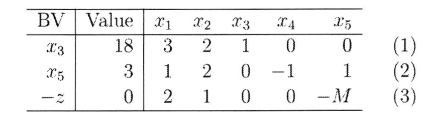When a Simplex step is performed and a artificial variable leaves the basis, it can be removed entirely from the tableau.

Duality

Seeing the original linear program as the primal program, the dual bounds the optimal value of the primal.

The coefficients of the objective function describe:

• In the Primal perspective: the contribution of products (revenue)
• In the Dual perspective: the value of capacity (shadow prices)

Thus, following the dual perspective, shadow prices can be used to calculate the firm’s value of a resource: $\text{Firm Value}=\text{Shadow Price}\ast \text{Capacity}$

Weak and Strong Duality

• Weak Duality Theorem: For any feasible solution of the primal and any feasible solution of the dual, the objective value of the primal is less than or equal to that of the dual.
• Strong Duality Theorem: If both the primal and dual have feasible solutions, then both have optimal solutions, and their objective values are equal at optimality.
• Unboundedness: If the primal is unbounded, the dual is infeasible, and vice versa.

• Dualizing twice yields the original primal.
• The shadow prices of the optimized dual are the negative production quantities of the primal
• The optimized dual is basically a transposed version of the optimized primal tableau

Complementary Slackness

This condition states that for each pair of primal and dual variables, at least one in the pair must be zero at optimality. This means that if the variable of the primal problem is in the basis, the slack variable of the associated dual constraint must be zero.

• Primal Variable > 0 → Dual Constraint is Binding (equality), = 0
• Primal Variable = 0 → Dual Constraint is Non-Binding (inequality), < 0

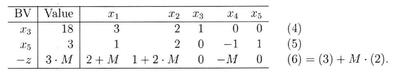
Dual Objective

The dual’s objective function is a minimization of each constraint’s capacity (right-hand side) multiplied by its shadow price (dual variable).

It’s constrained by each products’s (primal variable) production factors (primal constraint coefficients) multiplied by the respective shadow prices, which must be greater than or equal to the product’s contribution to the objective function (primal objective coefficient).

Primal	Dual

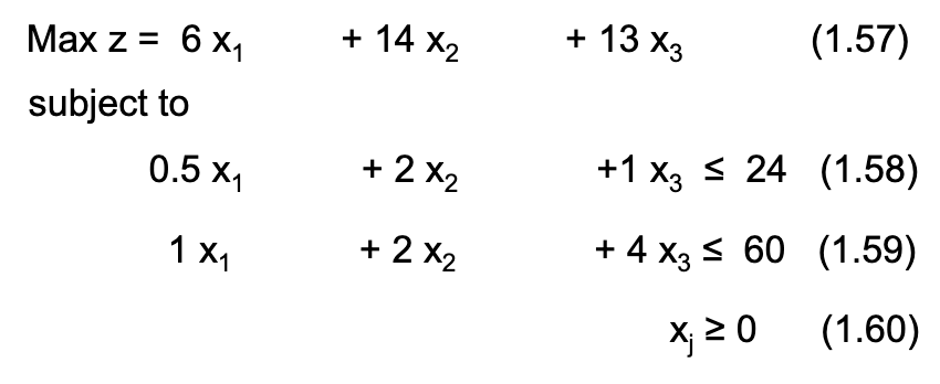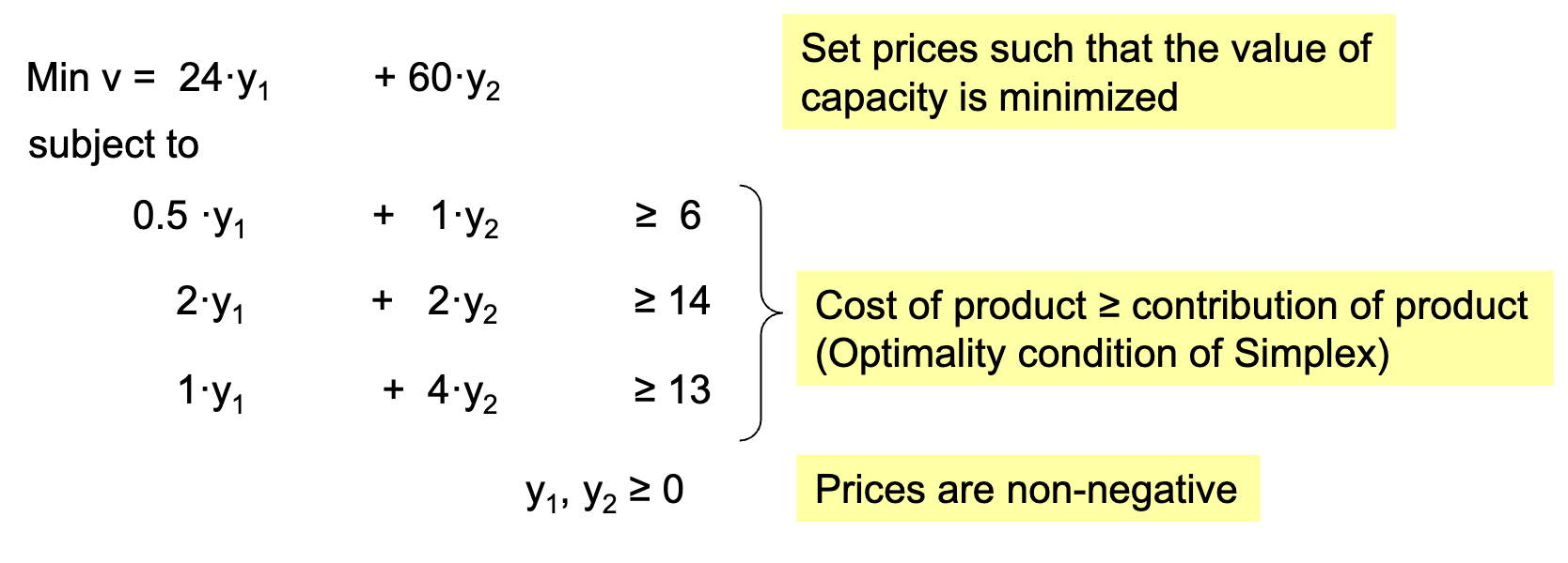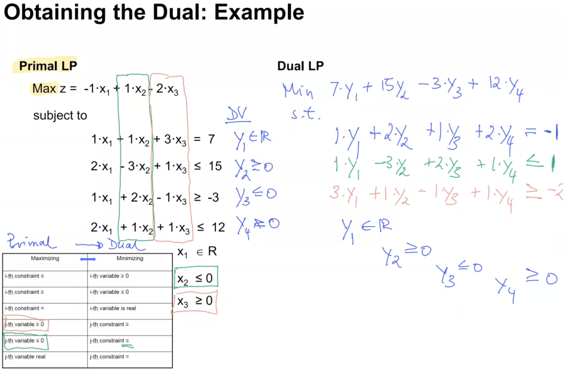
Obtaining the Dual

Maximizing (usually Primal)	Minimizing (usually Dual)
i-th constraint ≤	i-th variable ≥ 0
i-th constraint ≥	i-th variable ≤ 0
i-th constraint =	i-th variable is real
j-th variable ≥ 0	j-th constraint ≥
j-th variable ≤ 0	j-th constraint ≤
j-th variable real	j-th constraint =

The objective function is made up of each constraint’s right-hand side multiplied by its respective dual variable (shadow price). Each constraint in the dual is formed by the coefficients of the respective primal variable multiplied by the dual variables, which must be greater than or equal to (for maximization primal) the primal variable’s objective function coefficient. In other words, the constraint matrix is transposed.

Each dual variable corresponds to a primal constraint, and each dual constraint corresponds to a primal variable. The dual variables are constrained based on the type of primal constraints, defined in the table above.

Shadow Price

Shadow prices and reduced costs are concepts from the duality theory to provide insights into the sensitivity of the optimal solution to changes in the constraints and objective function coefficients.

The shadow price is the “value” of one additional unit of a resource in the constraints. It indicates the change in the objective function if the right-hand side of a constraint is increased by one unit (sometimes also called opportunity cost).

Each binding variable has its own shadow price. Non-binding variables have a shadow price of zero, as they do not limit the optimal solution.

Identifying Binding Constraints

Binding constraints directly affect the optimal solution, while non-binding constraints do not.

• A constraint is binding if its slack or surplus variable is zero in the optimal solution.
• Binding constraints have a shadow price greater than zero, while non-binding constraints have a shadow price of zero.

• $\le$ constraints have positive shadow prices in max problems, negative in min.
• $\ge$ constraints have negative shadow prices in max problems, positive in min.
• In all cases, the algebraic sign of the shadow price equals the domain of a dual variable.

Shadows prices can be read in an optimal tableau as the coefficients of the slack/surplus variable associated with the respective constraint in the objective function row.

Reduced Cost

Opposing shadow prices, the reduced cost measures the decrease in the objective function’s value if a non-basic variable is increased from $0$ to $1$. Reduced cost is the coefficient for the respective non-basic variable in the objective function row of the final optimized tableau.

• For a max problem, the reduced cost of a non-basic variable is negative and that of basic variables zero.
• In the special case of multiple optima solutions, some non-basic variables have zero reduced cost.

Pricing Out

Pricing out is the process of calculating reduced cost using shadow prices.
This may be useful when adding a new variable to an existing optimal solution. In this case, pricing out determines if the new variable is economically attractive compared to its opportunity cost (shadow prices).
It is the difference between its marginal benefit and the total shadow price value of the resources it uses.

${\bar{c}}_j=c_j-{\sum }_{i=1}^m(a_{ij}\times y_i)$

where $c_j$: j’s objective function coefficient (initial function), $a_{ij}$: amount of resource $i$ required to produce one unit of $x_j$, $y_i$: shadow price of constraint $i$.

Reduced cost can be read in an optimal tableau as the coefficient of the original decision variable.

Dual Simplex Method

The dual simplex method is used when the current solution is dual‑feasible but primal‑infeasible.

Unlike forming and solving the dual explicitly, the method operates directly on the primal tableau using modified pivot rules that restore primal feasibility while maintaining dual feasibility.

Step 1: Form the Primal Simplex Tableau
Set up the LP in a standard simplex tableau as usual.

The key requirement for starting dual simplex is:

• Reduced costs must satisfy dual feasibility (i.e., the optimality row is valid)
• Some RHS (basic variable values) may be negative → primal infeasibility

Step 2: Identify the Leaving Variable (Primal Infeasibility)
Select the row whose RHS value is most negative.
This row corresponds to a basic variable violating primal feasibility and must leave the basis.

Step 3: Determine the Entering Variable (Maintain Dual Feasibility)
From that row, consider only the columns with negative coefficients (since pivoting on these preserves dual feasibility).

For each such column $j$, compute the dual ratio (coefficient/shadow price divided by the selected right-hand side):
$\min \left\{\left|\frac{c_j}{a_{ij}}\right|:a_{ij}<0\right\}$

The entering variable is the one achieving the minimum ratio.

Here:

• $a_{ij}$ is the coefficient in the leaving row $i$ and candidate entering column $j$.
• $c_j$ is the reduced cost (objective row coefficient) associated with variable $x_j$.

Step 4: Pivot and Repeat
Perform the pivot, just like in the primal Simplex Algorithm.
This moves the solution closer to primal feasibility while keeping dual feasibility intact.

• Optimal: If all RHS are ≥ 0, the solution is optimal.
• Continue pivoting: If some RHS < 0, pick that row and try to pivot on a negative entry.
• Infeasible: If a row has RHS < 0 but no negative values, no pivot is possible → the problem is infeasible.

Special Cases

No Feasible Solution

A linear program with an infeasible solution occurs when there is no point that satisfies all constraints simultaneously; constraints conflict. This is detected during the two-phase method or the Big-M method when artificial variables cannot be driven to zero.

Unbounded Solution

When the objective function can increase indefinitely without violating any constraints, the linear program is unbounded. This is detected during the Simplex algorithm when all coefficients in the column of an entering variable are negative.

Redundant Constraint

A redundant constraint does not affect the feasible region because it is implied by other constraints. Removing it does not change the solution set; it is outside of the feasible region. This can be identified during sensitivity analysis, or when two constraints visibly overlap.

Primal Degeneracy

Primal degeneracy means that a basic feasible solution has one or more basic variables equal to zero. This can lead to cycling in the Simplex algorithm, where the algorithm revisits the same basic feasible solutions repeatedly without making progress toward optimality.

Identified when the leaving variable has a RHS value of zero, meaning that the pivot does not change the objective function value, and the algorithm may revisit the same solution.

Multiple Optimal Solutions: Dual Degeneracy

This occurs when the objective function line is parallel to a constraint line in the dual problem, leading to multiple optimal solutions. In the primal problem, this corresponds to having multiple basic feasible solutions that yield the same optimal objective value.

This can be seen when a non-basic variable has a reduced cost of zero in the optimal tableau; it could enter the basis without changing the objective value.

In the exam, there’s often a question on one of the special cases.

Sensitivity Analysis

Sensitivity analysis examines how the optimal solution changes in response to variations in the parameters of the linear programming model, such as objective function coefficients. Changes in constraints are more complex and not covered in this module.

This assumes that only one parameter is changed at a time, and the other parameters remain constant.

Optimality Range for Basic Variables

The objective here is to determine how much the objective function coefficient can be changed without changing the basis.

Identify the row of the variable for which the profit is changed (e..g $x1$) by and amount $\Delta$. Then, subtract a parameter $\Delta$ to each non-basic variable’s coefficient in the objective function row of the optimal tableau, multiplied by the respective column coefficient in the variable’s row.
The resulting expressions must remain $\le 0$ for optimality, which, combined, give the optimality range for $\Delta$.

$$0\le {\bar{c}}_k-(\Delta \times {\bar{a}}_{row,k})\le 0$$

This is subtraction and $\le$ because we’re using maximization problems in this lecture. For minimization problems, the signs would be reversed.

See slide 152

Optimality Range for Non-Basic Variables

Changes in objective function coefficients are directly reflected in the currently optimal tableau (by the same amount).

• The coefficient of non-basic variables is already negative in the optimal tableau. If it decreases further in, it stays negative and therefore non-basic.
• For the variable to become basic, the optimal tableau coefficient would have to become positive, which means the objective function coefficient must not increase by more than the current optimal value. In this case, the Simplex algorithm must be reapplied to find the new optimal solution.

$0\le {\bar{c}}_k+\Delta \le 0⟹\Delta \le |{\bar{c}}_k|$