Consumption and Demand

Resources

• Slides
• Exercise Slides, Solution

Common Function Types

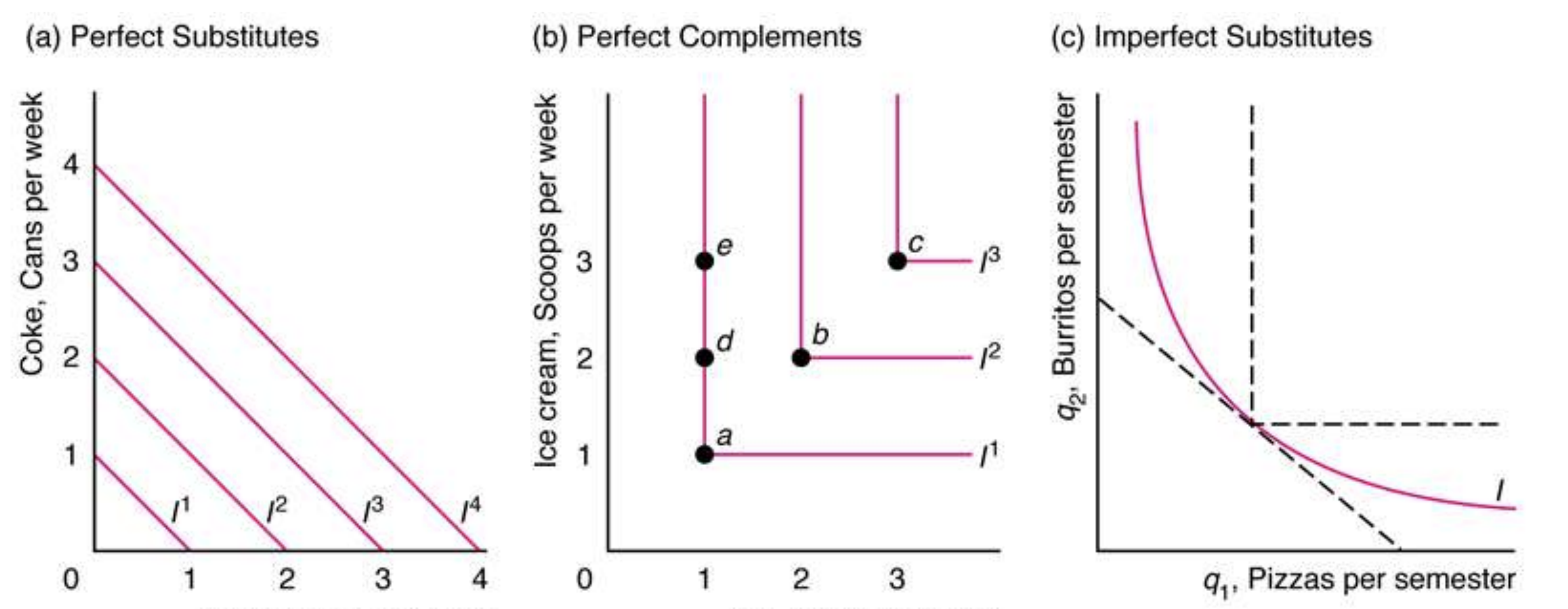
Perfect Substitutes

Two goods that an individual is willing to substitute at a constant rate. A linear utility function representing perfect substitutes has the form:

$$U(q_1,q_2)=a{q}_1+b{q}_2$$

• $a$ and $b$ are positive constants that represent the marginal utility of each good.
• The MRS is constant and equal to the ratio of the marginal utilities; indifference curve is linear (p. 9)

MRS for Perfect Substitutes

$$MR{S}_{1,2}=\frac{a}{b}$$

Optimal Consumption for Perfect Substitutes

The optimal consumption bundle depends on the price ratio.

If one good is cheaper per unit of utility, the individual will consume only that good. Otherwise, they are indifferent among all combinations on the budget line.

$$MR{S}_{1,2}=\{\begin{array}{ll}\text{If }\frac{p_1}{p_2}<\frac{a}{b},& \text{consume only good 1: }(q_1^{\ast },q_2^{\ast })=\left(\frac{y}{p_1},0\right)\\ \text{If }\frac{p_1}{p_2}>\frac{a}{b},& \text{consume only good 2: }(q_1^{\ast },q_2^{\ast })=\left(0,\frac{y}{p_2}\right)\\ \text{If }\frac{p_1}{p_2}=\frac{a}{b},& \text{any combination on the budget line is optimal}\end{array}$$

Perfect Complements

Two goods that an individual prefers to consume in a fixed proportion. Perfect complement functions are orthogonal (L-shaped) and have the form:

$$U(q_1,q_2)=\min \{a{q}_1,b{q}_2\}$$

• $a$ and $b$ are positive constants that determine the fixed proportion in which the goods are consumed.
• The MRS is either zero or infinite, depending on which good is in excess.
• The indifference curves are orthogonal (L-shaped). (p. 9)
• No substitution occurs between the goods.

MRS for Perfect Complements

If the first good is in excess, the MRS is 0; if the second good is in excess, the MRS is infinite.

$$MR{S}_{1,2}=\{\begin{array}{ll}0,& \text{if }a{q}_1>b{q}_2\\ \infty ,& \text{if }a{q}_1<b{q}_2\end{array}$$

Optimal Consumption for Perfect Complements

The optimal consumption bundle occurs where the goods are consumed in the fixed proportion.

$$\frac{q_1}{a}=\frac{q_2}{b}$$

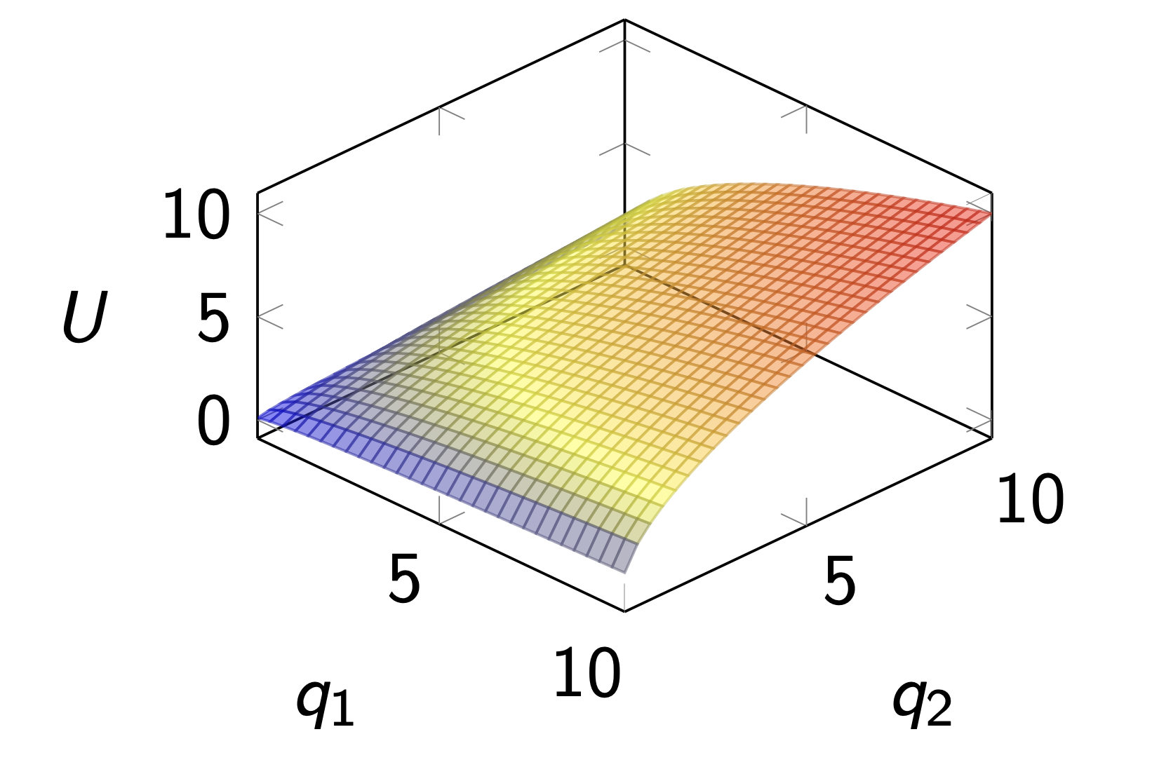
Cobb-Douglas

A common type of function used for modeling utility is the Cobb-Douglas function, which has the form:

$$U(q_1,q_2)=q_1^{\alpha }\cdot q_2^{\beta }$$

• $\alpha$ and $\beta$ are positive constants that determine the relative importance of each good to the individual.
• The Cobb-Douglas function exhibits diminishing marginal utility for each good and ensures that both goods are always consumed in positive quantities at the optimum.
• Cobb-Douglas Functions have no cross-price effects and therefore always yield ordinary goods.

MRS for Cobb-Douglas Functions

The Marginal Rate of Substitution (MRS) for a Cobb-Douglas utility function is given by:

$$MR{S}_{1,2}=\frac{\alpha }{\beta }\cdot \frac{q_2}{q_1}$$

Optimal Consumption for Cobb-Douglas

The quantity of each good consumed at the optimum can be derived as:

$$\begin{array}{rl}{q}_1^{\ast }& =\frac{\alpha }{\alpha +\beta }\cdot \frac{y}{p_1}\\ & \\ q_2^{\ast }& =\frac{\beta }{\alpha +\beta }\cdot \frac{y}{p_2}\end{array}$$

Quasilinear

Quasilinear functions are functions where one good is linear and the other is non-linear, represented as:

$$U(q_1,q_2)=f(q_1)+a{q}_2$$

• $f(q_1)$ is a concave function representing the utility derived from good 1.
• Good 2 is linear, meaning its marginal utility is constant.
• Quasilinear functions imply that the income effect only affects the consumption of the linear good (good 2).
• This is often used a luxury (nonlinear) and a necessity good (linear).

MRS for Quasilinear Functions

Since the partial derivative of good 2 is constant ($a$):

$$MR{S}_{1,2}=\frac{f^{\prime }(q_1)}{a}$$

Optimal Consumption for Quasilinear

The optimal consumption bundle can be found by solving:

$$\frac{f^{\prime }(q_1)}{a}=\frac{p_1}{p_2}$$

Once $q_1^{\ast }$ is determined, $q_2^{\ast }$ can be found using the budget constraint:

$$q_2^{\ast }=\frac{y-p_1{q}_1^{\ast }}{p_2}$$

This shows that the consumption of good 2 adjusts based on the remaining budget after purchasing good 1.

Optimal Consumption

Model Framework

• A representative individual derives utility from consuming two goods, $q_1$ and $q_2$.
• The individual is a price taker, meaning they accept the market prices $p_1$ and $p_2$ as given.
• The individual’s budget, $y$, is given and fixed. (p. 3)

Budget Constraint

Budget Line

• The budget line represents all consumption bundles $(q_1,q_2)$ that the individual can purchase by spending their entire budget. (p. 4)
• Equation: $y=p_1{q}_1+p_2{q}_2$
• This can be rearranged to show the quantity of good 2 as a function of good 1: $q_2=\frac{y}{p_2}-\frac{p_1}{p_2}{q}_1$
  • The slope of the budget line is the negative price ratio, $-\frac{p_1}{p_2}$.
  • The intercepts are the maximum affordable quantities of each good: $\frac{y}{p_1}$ and $\frac{y}{p_2}$.

Price Ratio

• The rate at which the individual can substitute one good for another at constant expenses. It represents the opportunity cost of consuming one good in terms of the other. (p. 4)
• Ratio: $\frac{p_1}{p_2}$

Utility

Utility Function

• A function $U(q_1,q_2)$ that represents an individual’s preference for different consumption bundles. (p. 5)
• Example: $U(q_1,q_2)=(q_1\cdot q_2{)}^{\frac{1}{2}}$
  
  

Indifference Curve

• A curve connecting all consumption bundles that provide the same level of utility. (p. 6)
• Higher indifference curves represent higher utility levels.
• The indifference curve is assumed to be transitive, monotonic, and convex.

Marginal Rate of Substitution (MRS)

• The rate at which an individual is willing to substitute one good for another while maintaining the same level of utility, therefore equals the price ratio. (p. 6)
• It is the absolute slope of the indifference curve at a given point.

$$MR{S}_{1,2}=\frac{\partial U/\partial q_1}{\partial U/\partial q_2}=\frac{p_1}{p_2}$$

Assumptions on Preferences

Assumptions about individual preferences ensure that utility functions and indifference curves behave in predictable ways. These assumptions include:

Completeness

• The individual can compare any two consumption bundles, A and B.
• For complete preferences, every consumption bundle lies on an indifference curve. (p. 7)

Transitivity

• If A is preferred to B, and B is preferred to C, then A must be preferred to C.
• If an individual is indifferent between A and B, and between B and C, they must be indifferent between A and C.
• Due to this, indifference curves cannot cross, which would imply a single point could provide different utility. (p. 7)

Monotonicity

• More of a good is always better.
• If bundle A contains more of at least one good and not less of the other than bundle B, A is at least as good as B ($A\succsim B$).
• If preferences are strictly monotonous, A is always better than B, and indifference curves are negatively sloped. (p. 8)

Convexity

• If an individual is indifferent between bundles A and B, any weighted average of A and B is at least as good as A or B.
• If preferences are strictly convex, any weighted average is strictly preferred, causing indifference curves to be “bowed inward”. (p. 8)
• Convexity: if $A\sim B$, then $\alpha A+(1-\alpha )B\succsim A\forall \alpha \in [0,1]$
• Strict convexity: if $A\sim B$, then $\alpha A+(1-\alpha )B\succ A\forall \alpha \in (0,1)$
• This shape reflects the assumption of diminishing marginal utility, meaning the more of a good a consumer has, the less additional satisfaction they get from each extra unit.

Utility Maximum

The Optimization Problem

The individual maximizes their utility function subject to their budget constraint. (p. 10)
\begin{flalign} \max_{q_1, q_2} & \quad U(q_1, q_2) &&\\ \text{s.t.} & \quad p_1q_1 + p_2q_2 \leq y && \end{flalign}

Interior Solution

An optimal consumption bundle $(q_1^{\ast },q_2^{\ast })$ within the budget (not on an axis) must satisfy two conditions:

1. The entire budget is spent: $p_1{q}_1+p_2{q}_2=y$
2. The slope of the indifference curve equals the slope of the budget line. This means the rate at which the individual is willing to trade goods equals the rate at which the market allows them to trade.
   $MR{S}_{1,2}=\frac{p_1}{p_2}$ (p. 10-11)

Photo Derivation

Lagrangian Method

Lagrangian Method

A technique used to find the maximum or minimum of a function subject to constraints. It introduces a new variable (the Lagrange multiplier) to convert the constrained optimization problem into an unconstrained one.

The Langrangian function $\mathcal{L}$ is set up as:

$\mathcal{L}(x_1,x_2,\lambda )=U(x_1,x_2)+\lambda (y-p_1{x}_1-p_2{x}_2)$

• $U(x_1,x_2)$ is the objective function (utility to be maximized).
• $\lambda$ (Lambda) is the Lagrange multiplier.
• $(yy-p_1{x}_1-p_2{x}_2)$ is the budget constraint for Budget $y$, rearranged so it equals zero at the optimal point. Since its $0$, adding $\lambda$ does not change the value but allows to use calculus for optimization.

Solving the Lagrangian

To maximize the Lagrangian function, the first order partial derivatives with respect to each variable ($x_1,x_2,\lambda$) are taken and set equal to 0. These first-order conditions (FOC) are:

1. $\frac{\partial \mathcal{L}}{\partial x_1}=\frac{\partial U}{\partial x_1}-\lambda p_1=0⟹{\mathbf{yU}}_1=\lambda p_1$
2. $\frac{\partial \mathcal{L}}{\partial x_2}=\frac{\partial U}{\partial x_2}-\lambda p_2=0⟹{\mathbf{yU}}_2=\lambda p_2$
3. $\frac{\partial \mathcal{L}}{\partial \lambda }=M-p_1{x}_1-p_2{x}_2=0⟹p_1{x}_1+p_2{x}_2=y$
   TThe system of equations is then solved for $x_1$ and $x_2$ as functions of the prices ($p_1,p_2$) and income ($M$). These solutions, ${\mathbf{x}}_1^{\ast }({\mathbf{p}}_1,{\mathbf{p}}_2,\mathbf{M})$ and ${\mathbf{x}}_2^{\ast }({\mathbf{p}}_1,{\mathbf{p}}_2,\mathbf{M})$, are the Marshallian demand functions.

Interpretation

• Condition 1 & 2: Optimal Allocation. This is the core principle of utility maximization: at the optimum, the marginal utility per dollar spent on all goods must be equal.
  Solving for $\lambda$ and setting the results equal yields:
  $\frac{M{U}_1}{p_1}=\frac{M{U}_2}{p_2}=\lambda$
• Condition 3: Budget Constraint. All income is spent on the optimal bundle.
• Lagrange Multiplier $\lambda$: Measures the marginal utility of income. It tells you how much the consumer’s maximum utility would increase if their income ($M$) were to increase by one dollar.

Factors Influencing Optimal Consumption

Change in Income

Normal vs. Inferior Goods

• Normal Good: Consumption increases as income increases ($\frac{\partial q_i}{\partial y}>0$). Indifference curves shift up-right parallelly to the budget line.
• Inferior Good: Consumption decreases as income increases ($\frac{\partial q_i}{\partial y}<0$). Indifference curves shift up-right but the consumption of the inferior good decreases.
  • Examples: Instant noodles, long-distance busses.

(p. 12)

Change in Prices

A change in the price of a good affects consumption in two ways: (p. 13)

Effects of a Price Change

• Substitution Effect: A change in the price ratio encourages the consumer to substitute the now relatively more expensive good with the cheaper one.
• Income Effect: A price change alters the individual’s purchasing power. A price drop increases purchasing power, while a price hike decreases it.

The total change in consumption is the sum of these two effects. (p. 14)

Types of Goods based on Price Changes

• Ordinary Good: Consumption decreases as its own price increases ($\frac{\partial q_i}{\partial p_i}<0$).
  • If the good is normal, the substitution and income effects work in the same direction.
  • If the good is inferior, the substitution effect is stronger than the income effect.
• Giffen Good: Consumption increases as its own price increases ($\frac{\partial q_i}{\partial p_i}>0$).
  • This is a rare case where the good must be inferior, and the income effect is stronger than the substitution effect. (p. 15)

Relationships Between Goods

• Substitutes: An increase in the price of good i causes an increase in the consumption of good j ($\frac{\partial q_j}{\partial p_i}>0$). The goods can replace each other.
• Complements: An increase in the price of good i causes a decrease in the consumption of good j ($\frac{\partial q_j}{\partial p_i}<0$). The goods are often used together.
  • A complementary good must be a normal good. (p. 16)

Higgsian Bundles

The Higgsian decomposition is a method used to separate the total effect of a price change into its substitution and income effects. It involves constructing a hypothetical budget line that reflects the new price ratio but keeps the consumer’s utility level constant.

First, the new, compensated consumption bundle is determined by finding the point on the new budget line that lies on the original indifference curve. The difference between the original consumption bundle and this compensated bundle represents the substitution effect.

At interior optima, the marginal rate of substitution (MRS) equal the (now new) price ratio:

$$MRS=\frac{p_1^{\prime }}{p_2^{\prime }}$$

This can then be used to substitute one demand function into the other and solve for the compensated bundle by setting it equal to the original utility level. The Higgsian bundle are the new quantities.

The substituion effect is the movement from the original optimum to the compensated bundle, the substitution effect is the difference the compensated bundle and the new optimum after the price change:

$$\begin{array}{rl}\text{Substitution Effect}& =q_i^H-q_i\\ \text{Income Effect}& =q_i^{\prime }-q_i^H\end{array}$$

Income Compensation

To calculate the new income required to keep the same utility level with new prices, simply multiply the Higgsian bundle determined like above with the new prices:

$$y^{\prime }=p_1^{\prime }\cdot q_1^H+p_2^{\prime }\cdot q_2^H$$

Individual and Market Demand

Individual Demand Curve

• The individual demand curve shows the quantity of a good that a single consumer will purchase at various prices, holding all other factors constant.
• For an ordinary good, this curve is downward sloping. (p. 17)

Market Demand

• Market demand is the horizontal summation of all individual demand curves for a good.
• It represents the total quantity demanded by all consumers in a market at each price.
• Equation: $Q=\sum q_i$ (p. 18)

Law of Demand

• The empirical observation that, ceteris paribus, as the price of a good increases, the quantity demanded decreases.
• This results in a downward-sloping market demand curve: $\frac{\partial Q}{\partial p}<0$ (p. 18)

Example Problem

This is the consumption & demand problem from exercise exam 1 with some questions from exercise exam 2 and exercise 2.

An individual with income $y>0$ and a utility function $U(q_1,q_2)=4q_1^{\frac{1}{2}}+2q_2$ consumes goods with prices $p_1>0$ and $p_2>0$.

Preparation

This is a quasilinear function.

Marginal Utilities and MRS:
The partial derivatives.

• $M{U}_1=(4q_1^{\frac{1}{2}}{)}^{\prime }=2q_1^{-\frac{1}{2}}$
• $M{U}_2=2$
• $MRS=q_1^{-\frac{1}{2}}$

Questions

What’s the optimal consumption?
Setting $MRS=\text{Price Ratio}$, or following the formula above:

$$q_1^{-\frac{1}{2}}=\frac{p_1}{p_2}⟹q_1^{\ast }={\left(\frac{p_2}{p_1}\right)}^2$$

which is subtracted from the budget constraint to find $q_2^{\ast }$:

$$q_2^{\ast }=\frac{y-p_1{\left(\frac{p_2}{p_1}\right)}^2}{p_2}=\frac{y}{p_2}-\frac{p_2}{p_1}$$

How can the goods be characterized?
This is about normal/inferior, ordinary/giffen, substitutes/complements.

• Good 1 is normal, the income has no effect on it. Therefore, it is also ordinary.
• Good 2 is normal, as the formula shows a positive relation with income. Therefore, it is also ordinary.
• Both goods are substitutes, as an increase in the price of one good increases the consumption of the other, as seen in the formulas.

How does the consumption change as the price of good 1 increases?

• Good 1 is normal, therefore, as price increases, consumption decreases.
• The goods are substitutes, therefore, as price of good 1 increases, consumption of good 2 increases.

In other words, as $p_1$ increases:

• $q_1^{\ast }$ decreases, as it is inversely proportional to the square of $p_1$.
• $q_2^{\ast }$ increases, as the second term $\frac{p_2}{p_1}$ decreases.

Assuming $y=200$, $p_1=1$, and $p_2=10$, what is the optimal consumption bundle?
Using the optimal consumption determined above:

• $q_1^{\ast }={\left(\frac{10}{1}\right)}^2=100$
• $q_2^{\ast }=\frac{200}{10}-\frac{10}{1}=20-10=10$

Under the same assumption, what’s the optimal spending per good?

• Spending on good 1: $p_1\cdot q_1^{\ast }=1\cdot 100=100$
• Spending on good 2: $p_2\cdot q_2^{\ast }=10\cdot 10=100$

Consider a price decrease to $p_2^{\prime }=5$. What’s the hypothetical consumption bundle, where the utility equals that of before the price decrease at minimum spending?
This is the Higgsian bundle. First, calculate the original utility: $U(100,10)=4\cdot 10+2\cdot 10=60$.
Now, set up the MRS with the new price ratio:

$$q_1^{-\frac{1}{2}}=\frac{p_1}{p_2^{\prime }}=\frac{1}{5}⟹q_1^H=25$$

Substituting into the utility function to find $q_2^H$:

$$60=4\cdot (25{)}^{\frac{1}{2}}+2q_2^H⟹60=20+2q_2^H⟹q_2^H=20$$

Thus, the Higgsian bundle is $(25,20)$.

What income would the individual need after the price decrease to reach the same utility as before?
Using the Higgsian bundle and the new prices:

$$y^{\prime }=p_1\cdot q_1^H+p_2^{\prime }\cdot q_2^H=1\cdot 25+5\cdot 20=25+100=125$$

Decompose price increase into substitution and income effects.
Original bundle: $(100,10)$
Higgsian bundle: $(25,20)$
New optimal bundle after price decrease, using the optimal consumption formulas: $(25,35)$

Good 1 has no income effect, as it is quasilinear.

Good	Substitution Effect	Income Effect
Good 1	$25-100=-75$	0
Good 2	$20-10=-10$	$35-20=15$

Approaches

• Individual Demand Functions: Partial Derivatives
• Optimal Consumption Bundle: MRS = Price Ratio ($\frac{p_1}{p_2}=\frac{q_1}{q_2}=MRS$)
• Characterizing Goods:
  • Normal/Inferior: $\frac{\partial q_i}{\partial y}>0$ / $\frac{\partial q_i}{\partial y}<0$, if price increases with income, good is normal
  • Ordinary/Giffen: $\frac{\partial q_i}{\partial p_i}<0$ / $\frac{\partial q_i}{\partial p_i}>0$, only inferior goods can be Giffen: income effect stronger than substitution effect
  • Substitutes/Complements: $\frac{\partial q_j}{\partial p_i}>0$ / $\frac{\partial q_j}{\partial p_i}<0$, complementary goods must be normal
• Decomposing Effects / Income After Price Change: Higgsian Bundle

Gemini Additions

Identifying Function Types at a Glance

• Cobb-Douglas Shortcut: For $U=q_1^{\alpha }{q}_2^{\beta }$, the expenditure share of good 1 is always $\frac{\alpha }{\alpha +\beta }$ of total income $y$. This saves time during Lagrangian derivations.
• Quasilinear Corner Solutions: In quasilinear problems (e.g., $U=\sqrt{q_1}+q_2$), always check if $y$ is large enough to afford the “optimal” $q_1^{\ast }$. If $y<p_1{q}_1^{\ast }$, the consumer has a corner solution: $q_1=y/p_1$ and $q_2=0$.

Lagrangian Check

• Marginal Utility per Dollar: Use the condition $\frac{M{U}_1}{p_1}=\frac{M{U}_2}{p_2}$ as a quick check for interior optima.
• Interpretation of $\lambda$: Remember that $\lambda =\frac{\partial U^{\ast }}{\partial y}$ (the “shadow price” of the budget constraint). It represents the utility gain from one additional unit of income.

Income & Substitution Effects (The Slutsky vs. Hicksian Nuance)

• Hicksian Decomposition (Constant Utility): 1. Calculate original utility $U_0$.
  2. Set $MRS=\text{new price ratio}$ to find the ratio of $q_1$ to $q_2$.
  3. Plug that ratio into the original utility function $U(q_1,q_2)=U_0$ to find the Higgsian bundle $(q_1^H,q_2^H)$.
• Slutsky Decomposition (Constant Purchasing Power): This involves adjusting income so the consumer can just afford the original bundle at new prices ($y^{\prime }=p_1^{\prime }{q}_1+p_2^{\prime }{q}_2$).

Demand Elasticities

• Price Elasticity of Demand: ${ϵ}_p=\frac{\partial Q}{\partial p}\cdot \frac{p}{Q}$. If $|ϵ|>1$, demand is elastic; if $|ϵ|<1$, it is inelastic.
• Income Elasticity: ${ϵ}_y=\frac{\partial Q}{\partial y}\cdot \frac{y}{Q}$. Positive for normal goods, negative for inferior goods.