Production and Supply

f> [!example] Resources

• Slides
• Exercise Slides, Solution

Context

• A company produces $q$ units of a single good, employing two inputs to production, labor $L$ and capital $K$.
• The firm is a price taker in both input prices for labor $w$ and capital $r$ as well as the output price $p$.
• Input costs: $c=wL+rK$
• Revenue: $R(q)=pq$

Assumptions on Production Technology (production function $F(L,K)$):

• Monotonicity: More inputs lead to more output. $F(L^{\prime },K^{\prime })\ge F(L,K)$ for $L^{\prime }\ge L$ and $K^{\prime }\ge K$.
• Convexity: The marginal products of inputs are diminishing. $F$ is a convex function (bowed outwards). If two input bundles yield the same output, any convex combination of these bundles yields at least the same output. If technology is strictly convex, so are the isoquants, and the same for non-strict convexity.

Optimization

Cost Minimization

The firm aims to minimize costs for a given output level $q$:

$$\underset{L,K\ge 0}{\min }wL+rK\text{s.t.}F(L,K)\ge q$$

Cost Minimization Condition

The firm minimizes costs by choosing input levels such that the input price ratio equals the marginal rate of technical substitution (MRTS).

$$MRT{S}_{L,K}=\frac{\partial F/\partial L}{\partial F/\partial K}=\frac{w}{r}$$

The Lagragian for this problem is given by:

$$\mathcal{L}(L,K,\lambda )=wL+rK+\lambda (q-F(L,K))$$

Change in Output

The curve describing how output changes with input levels. To increase output, at least one input must be increased, and vice versa. See slide 12.

Profit Maximum

The firm aims to maximize profit (a function of output and total costs) by maxizing its output::

$$\underset{q}{\max }\pi (q)=R(q)-C(q)$$

where $R(q)$ is the revenue function and $C(q)$ the cost function.

Profit Maximization Condition

The firm maximizes profit by producing the output level where marginal revenue $MR$ equals marginal costs $MC$:

$$\begin{array}{rl}MR(q)& =MC(q)\\ & \\ \frac{dR(q)}{dq}& =\frac{dC(q)}{dq}\end{array}$$

For a price-taking firm, marginal revenue equals the output price $p$, so that an optimal solution requires $p=MC(q)$. The firm produces output as long as the price covers marginal costs.

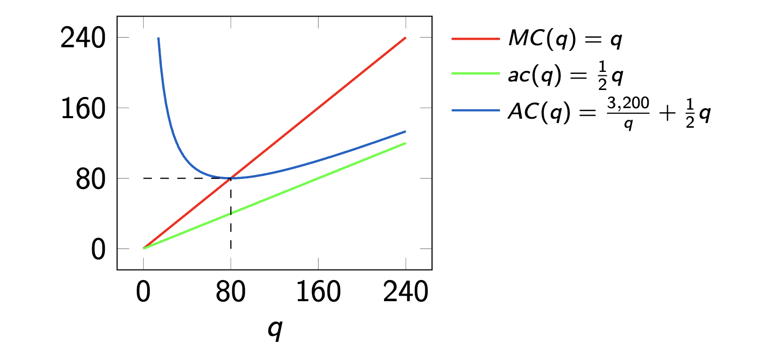
Marginal Cost Curve

The curve describing how marginal costs change with output level $q$. As costs are assumed to be strictly convex, marginal costs increase with output, and vice versa. See slide 17.

An increase in the output price $p$ (and therefore $MC$ for price-taking firms) leads to a higher optimal output level, and vice versa.

Terms

Production Function

Similar to the utility function for consumers. The production function $F(L,K)$ describes the maximum output $q$ the firm can produce from the given input bundle $(L,K)$. It can be seen as the firm’s technology.

Input Price Ratio

The rate at which the firm can trade one input for another at constant input costs is given by the input price ratio: $\frac{w}{r}$

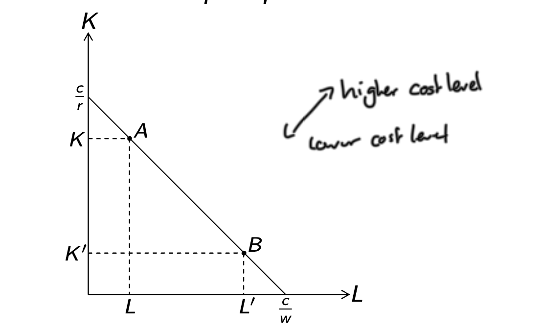
Isocost Line

The line representing all combinations of inputs that yield the same total cost $c$ is called an isocost line.
It is given by the cost equation rearranged for $K$: $K=\frac{c}{r}-\frac{w}{r}L$
Its slope is given by the negative input price ratio: $-\frac{w}{r}$.

Marginal Rate of Technical Substitution (MRTS)

The rate at which the firm can substitute one input for another while keeping output constant is given by the marginal rate of technical substitution (MRTS):

$$MRT{S}_{L,K}=-\frac{dK}{dL}{|}_{q\text{ constant}}=\frac{M{P}_L}{M{P}_K}$$

where $M{P}_L=\frac{\partial F(L,K)}{\partial L}$ and $M{P}_K=\frac{\partial F(L,K)}{\partial K}$ are the marginal products of labor and capital, respectively.

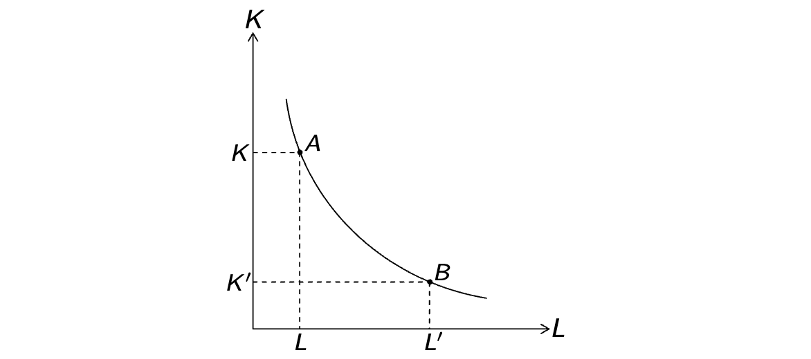
Isoquant

The curve representing all combinations of inputs that yield the same output level $q$ is called an isoquant.
Its slope is given by the negative MRTS: $-\frac{M{P}_L}{M{P}_K}$.

For perfect substitutes, the isoquants are straight lines. For perfect complements, they are L-shaped. Otherwise, they are convex curves.

• The isoquant is downward sloping if $M{P}_L,M{P}_K>0$ (more inputs lead to more output). This is required by the monotonicity assumption.
• The isoquant is convex if $\frac{{\partial }^{2}F}{\partial L^2},\frac{{\partial }^{2}F}{\partial K^2}<0$ (diminishing marginal products). This is required by the convexity assumption.

Returns to Scale

Describes how output changes when all inputs are scaled by the same factor.

• Increasing Returns to Scale: Doubling inputs more than doubles output. $F(\lambda L,\lambda K)>\lambda F(L,K)$ for $\lambda >1$.
• Decreasing Returns to Scale: Doubling inputs less than doubles output. $F(\lambda L,\lambda K)<\lambda F(L,K)$ for $\lambda >1$.
• Constant Returns to Scale: Doubling inputs exactly doubles output. $F(\lambda L,\lambda K)=\lambda F(L,K)$ for $\lambda >0$.

Production Costs

Production costs are divided into fixed costs $c^f$ and variable costs $c(q)$. Fixed costs are independent of output, while the variable costs function represents the minimum input costs given output $q$.

• Total Costs $C(q)$: The sum of fixed and variable costs: $C(q)=c^f+c(q)$
• Average Costs $AC(q)$: The total costs per unit of output: $AC(q)=\frac{C(q)}{q}$.
• Average Variable Costs $AVC(q)$: The variable costs per unit of output: $AVC(q)=\frac{c(q)}{q}$.
  In the notes, $AVC$ is referred to as lower-case $ac$.
• Marginal Costs $MC(q)$: The additional total costs of producing one more unit of output: $MC(q)=\frac{dC(q)}{dq}=\frac{dc(q)}{dq}$.

Variable Cost Curve

The curve describing how variable costs change with output level $q$. As output increases, variable costs increase, and vice versa. The price of capital is normalized to $r=1$. See slide 14.

Short-Run vs. Long-Run Costs

• Short-Run Total Costs: In the short run, fixed costs are sunk costs, and must be considered in total costs: $C_{SR}(q)=c^f+c_{SR}(q)$.
• Long-Run Total Costs: In the long run, non-variable costs are quasi-fixed; meaning they are only considered if the firm operates:

C_{LR} = \begin{cases}
c^f + c_{LR}(q) & \text{if } q > 0\
0 & \text{if } q = 0
\end{cases}

Supply Terms

Optimal Production

The firm either supplies an optimal output $q>0$ satisfying $p=MC(q)$, or no output $q=0$.

• In the short run, the firm only supplies $q>0$ if the output price covers average variable costs: $p\ge AVC(q)⟺R(q)\ge c(q)$.
• In the long run, the firm only supplies $q>0$ if the output price covers average total costs: $p\ge AC(q)⟺R(q)\ge C(q)$.

Individual Supply Curve

The individual supply curve refers to the marginal cost curve (price per output) above the cost line.

• In the short term, marginal cost $MC$ has to exceed the average variable costs $AVC$
• In the long term, marginal cost $MC$ has to exceed the average total costs $AC$

Here, the individual supply curve begins at $q=0$ in the short term, or $q=80$ in the long term.

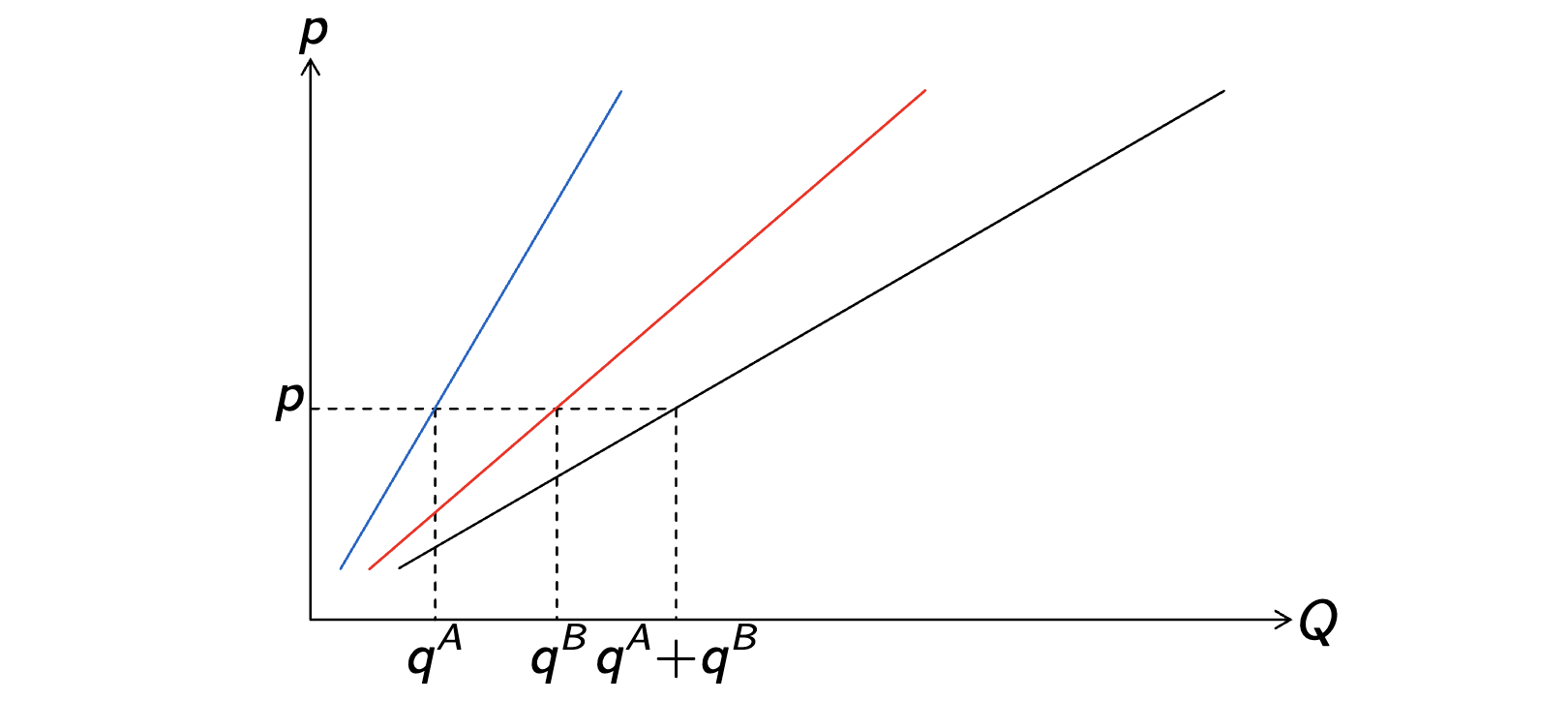
Market Supply Curve

The market supply curve is the horizontal sum of all individual supply curves in the market. That is, the supply at a given price for a single good across all firms.

$$Q=\sum q$$

Here, black is the market supply curve, summing up the individual supply curves of firms A and B.

Law of Supply

There is a positive relationship between price and quantity supplied. As price increases, quantity supplied increases, and vice versa. This is because higher prices allow firms to cover higher marginal costs.

Common Function Types

Precomputed properties of common production functions. The corresponding consumption functions are explained more in consumption and demand.

Cobb-Douglas Production Function

The Cobb-Douglas production function is given by:

$$F(L,K)=A{L}^{\alpha }{K}^{\beta }$$

Marginal Products and MRTS for Cobb-Douglas

$$\begin{array}{rl}M{P}_L& =A\alpha L^{\alpha -1}{K}^{\beta }\\ & \\ M{P}_K& =A\beta L^{\alpha }{K}^{\beta -1}\\ & \\ MRT{S}_{L,K}& =\frac{\alpha }{\beta }\cdot \frac{K}{L}\end{array}$$

Optimal Input Bundle for Cobb-Douglas

$$\begin{array}{rl}{L}^{\ast }& ={\left(\frac{r}{w}\cdot \frac{\alpha }{\beta }\right)}^{\frac{\beta }{\alpha +\beta }}\cdot {\left(\frac{q}{A}\right)}^{\frac{1}{\alpha +\beta }}\\ & \\ K^{\ast }& ={\left(\frac{w}{r}\cdot \frac{\beta }{\alpha }\right)}^{\frac{\alpha }{\alpha +\beta }}\cdot {\left(\frac{q}{A}\right)}^{\frac{1}{\alpha +\beta }}\end{array}$$

Returns to Scale for Cobb-Douglas

When inputs change by factor $\lambda$, output changes by factor ${\lambda }^{\alpha +\beta }$

• Increasing Returns to Scale if $\alpha +\beta >1$
• Constant Returns to Scale if $\alpha +\beta =1$
• Decreasing Returns to Scale if $\alpha +\beta <1$

Isoquants are strictly convex

Production Costs for Cobb-Douglas

Variable costs are given by:

$$c(q)=K{q}^{\frac{1}{\alpha +\beta }}\text{with}K={\left(\frac{w^{\beta }{r}^{\alpha }}{A^{\alpha +\beta }}\right)}^{\frac{1}{\alpha +\beta }}\cdot (\alpha +\beta )\cdot {\left(\frac{1}{{\beta }^{\beta }{\alpha }^{\alpha }}\right)}^{\frac{1}{\alpha +\beta }}$$

Simplified Cobb-Douglas Production Function

The simplified Cobb-Douglas production function is often used in exams and assumes equal exponents and $A=1$:

$$F(L,K)=(LK{)}^{\alpha }$$

Marginal Products and MRTS for Simplified Cobb-Douglas

$$\begin{array}{rl}M{P}_L& =\alpha L^{\alpha -1}{K}^{\alpha }\\ & \\ M{P}_K& =\alpha L^{\alpha }{K}^{\alpha -1}\\ & \\ MRT{S}_{L,K}& =\frac{K}{L}\end{array}$$

Optimal Input Bundle for Simplified Cobb-Douglas

$$\begin{array}{rl}{L}^{\ast }& ={\left(\frac{r}{w}\right)}^{\frac{1}{2}}\cdot q^{\frac{1}{2\alpha }}\\ & \\ K^{\ast }& ={\left(\frac{w}{r}\right)}^{\frac{1}{2}}\cdot q^{\frac{1}{2\alpha }}\end{array}$$

Here, labor and capital are always used in equal proportions.

Returns to Scale for Simplified Cobb-Douglas

When inputs change by factor $\lambda$, output changes by factor ${\lambda }^{2\alpha }$

• Increasing Returns to Scale if $\alpha >0.5$
• Constant Returns to Scale if $\alpha =0.5$
• Decreasing Returns to Scale if $\alpha <0.5$

Isoquants are strictly convex

Production Costs for Simplified Cobb-Douglas

Variable costs are given by:

$$c(q)=K{q}^{\frac{1}{2\alpha }}\text{with}K=2{\left(wr\right)}^{\frac{1}{2}}\cdot {\left(\frac{1}{{\alpha }^{\alpha }(1-\alpha {)}^{1-\alpha }}\right)}^{\frac{1}{2\alpha }}$$

Linear Production Function

Also called perfect substitutes production function and similar to the perfect substitutes demand function. Given by:

$$F(L,K)=aL+bK$$

Marginal Products and MRTS for Linear

$$\begin{array}{rl}M{P}_L& =a\\ & \\ M{P}_K& =b\\ & \\ MRT{S}_{L,K}& =\frac{a}{b}\end{array}$$

Optimal Input Bundle for Linear

• If $\frac{w}{r}>\frac{a}{b}$: $L^{\ast }=0$, $K^{\ast }=\frac{q}{b}$
• If $\frac{w}{r}<\frac{a}{b}$: $L^{\ast }=\frac{q}{a}$, $K^{\ast }=0$
• If $\frac{w}{r}=\frac{a}{b}$: any combination on the isoquant is optimal

Only the product where the input price ratio is lower than the MRTS is used, unless they are equal.

Returns to Scale for Linear

When inputs change by factor $\lambda$, output changes by factor $\lambda$.
Constant returns to scale.
Isoquants are linear

Production Costs for Linear

Variable costs are given by:

$$c(q)=\{\begin{array}{ll}\frac{w}{a}q& \text{if }\frac{w}{r}<\frac{a}{b}\\ & \\ \frac{r}{b}q& \text{if }\frac{w}{r}>\frac{a}{b}\\ & \\ \min \left\{\frac{w}{a},\frac{r}{b}\right\}q& \text{if }\frac{w}{r}=\frac{a}{b}\end{array}$$

Fixed Proportions Production Function

Also called Leontief production function and similar to the perfect complements demand function. Given by:

$$F(L,K)=\min \left\{\frac{L}{a},\frac{K}{b}\right\}$$

Marginal Products and MRTS for Fixed Proportions

Condition	$M{P}_L$	$M{P}_K$	$MRT{S}_{L,K}$
$\frac{L}{a}<\frac{K}{b}$	$\frac{1}{a}$	$0$	$\infty$
$\frac{L}{a}>\frac{K}{b}$	$0$	$\frac{1}{b}$	$0$
$\frac{L}{a}=\frac{K}{b}$	undefined	undefined	undefined

The marginal products and MRTS depend on the input ratio. When inputs are not in the fixed proportion, only one input has a positive marginal product.
When the inputs are in fixed proportion ($\frac{L}{a}=\frac{K}{b}$), these are undefined because the isoquant has a kink where both inputs need to be increased to increase output.

Optimal Input Bundle for Fixed Proportions

$$\begin{array}{rl}{L}^{\ast }& =aq\\ & \\ K^{\ast }& =bq\end{array}$$

The optimal input bundle is always in the fixed proportion.

Returns to Scale for Fixed Proportions

When inputs change by factor $\lambda$, output changes by factor $\lambda$.
Constant returns to scale.
Isoquants are L-shaped

Simplified Constant Elasticity of Substitution (CES) Production Function

A simplified version of the CES production function often used in exams, assuming equal weights and $A=1$. Given by:

$$F(L,K)=L^{\alpha }+K^{\alpha }$$

Marginal Products and MRTS for Simplified CES

$$\begin{array}{rl}M{P}_L& =\alpha L^{\alpha -1}\\ & \\ M{P}_K& =\alpha K^{\alpha -1}\\ & \\ MRT{S}_{L,K}& =\frac{M{P}_L}{M{P}_K}={\left(\frac{L}{K}\right)}^{\alpha -1}\end{array}$$

Optimal Input Bundle for Simplified CES

$$\begin{array}{rl}{L}^{\ast }& ={\left(\frac{w}{r}\right)}^{\frac{1}{\alpha -1}}{\left(\frac{q}{1+{\left(\frac{w}{r}\right)}^{\frac{\alpha }{\alpha -1}}}\right)}^{\frac{1}{\alpha }}\\ & \\ K^{\ast }& ={\left(\frac{q}{1+{\left(\frac{w}{r}\right)}^{\frac{\alpha }{\alpha -1}}}\right)}^{\frac{1}{\alpha }}\end{array}$$

Returns to Scale for Simplified CES

When inputs change by factor $\lambda$, output changes by factor ${\lambda }^{\alpha }$

• Increasing Returns to Scale if $\alpha >1$
• Constant Returns to Scale if $\alpha =1$
• Decreasing Returns to Scale if $0<\alpha <1$

Isoquants are strictly convex when $0<\alpha <1$

Production Costs for Simplified CES

Variable costs are given by:

$$c(q)=K{q}^{\frac{1}{\alpha }}\text{with}K={\left(\frac{1}{1+{\left(\frac{w}{r}\right)}^{\frac{\alpha }{\alpha -1}}}\right)}^{\frac{1}{\alpha }}\left[w{\left(\frac{w}{r}\right)}^{\frac{1}{\alpha -1}}+r\right]$$

Example Problem 2

This is the production & supply problem from exercise exam 1 with questions from exercise 3 and exercise exam 2.

A firm has the production function: $q=F(L,K)=(LK{)}^{\frac{1}{4}}$ and achieves an output of $q=10$.

Preparation

Marginal Products and MRTS:

• $M{P}_L=\frac{\partial F}{\partial L}=\frac{1}{4}{L}^{-\frac{3}{4}}{K}^{\frac{1}{4}}$
• $M{P}_K=\frac{\partial F}{\partial K}=\frac{1}{4}{L}^{\frac{1}{4}}{K}^{-\frac{3}{4}}$
• $MRT{S}_{L,K}=\frac{M{P}_L}{M{P}_K}=\frac{K}{L}$

Questions: Cost Minimization

What is the optimal production bundle to minimize cost?
For this, the MRTS (marginal rate of technical substitution) must equal the input price ratio:

$$\begin{array}{rl}MRT{S}_{L,K}& =\frac{w}{r}\\ & \\ \frac{K}{L}& =\frac{w}{r}\\ & \\ K& =\frac{w}{r}L\end{array}$$

Then, to find the optimal input bundle as a function of output $q$, substitute $K$ into the production function and solve for $L$:

$$\begin{array}{rl}q& =(LK{)}^{\frac{1}{4}}\\ & \\ q& ={\left(L\cdot \frac{w}{r}L\right)}^{\frac{1}{4}}\\ & \\ q^4& =\frac{w}{r}{L}^2\\ & \\ L^{\ast }& ={\left(\frac{r}{w}\right)}^{\frac{1}{2}}{q}^2\end{array}$$

Substituting $L^{\ast }$ back to find $K^{\ast }$:

$$\begin{array}{rl}{K}^{\ast }& =\frac{w}{r}{L}^{\ast }\\ & \\ K^{\ast }& =\frac{w}{r}{\left(\frac{r}{w}\right)}^{\frac{1}{2}}{q}^2\\ & \\ K^{\ast }& ={\left(\frac{w}{r}\right)}^{\frac{1}{2}}{q}^2\end{array}$$

What is the variable cost function $c(q)$?
Using the optimal input bundle formulas derived above, we can express the cost function as:

$$\begin{array}{rl}c(q)& =w{L}^{\ast }+r{K}^{\ast }\\ & \\ & =w{\left(\frac{r}{w}\right)}^{\frac{1}{2}}{q}^2+r{\left(\frac{w}{r}\right)}^{\frac{1}{2}}{q}^2\\ & \\ & =\left(w{w}^{-\frac{1}{2}}{r}^{\frac{1}{2}}+r{r}^{-\frac{1}{2}}{w}^{\frac{1}{2}}\right)q^2\\ & \\ & =2(wr{)}^{\frac{1}{2}}{q}^2\end{array}$$

What is the marginal cost function $MC(q)$?
Simply derive the variable cost function (fixed costs would vanish in derivation):

$$\begin{array}{rl}MC(q)& =\frac{dc(q)}{dq}\\ & \\ & =\frac{d}{dq}\left(2(wr{)}^{\frac{1}{2}}{q}^2\right)\\ & \\ & =4(wr{)}^{\frac{1}{2}}q\end{array}$$

If $w$ increases from $w=5$ to $w=20$, with r constant at $5$, calculate the cost increase for the optimal input after the change.

Using the optimal input bundle formulas derived above, we can calculate the optimal inputs before and after the price change.

• Before: $L={\left(\frac{5}{5}\right)}^{\frac{1}{2}}10^2=100$, $K={\left(\frac{5}{5}\right)}^{\frac{1}{2}}10^2=100$
• After: $L={\left(\frac{5}{20}\right)}^{\frac{1}{2}}10^2=70.71$, $K={\left(\frac{20}{5}\right)}^{\frac{1}{2}}10^2=200$

Then calculate the costs before and after the price change:

• Cost before: $c=wL+rK=5\cdot 100+5\cdot 100=1000$
• Cost after: $c=20\cdot 70.71+5\cdot 200=1414.2+1000=2414.2$
• Cost increase: $2414.2-1000=1414.2$

Questions: Production Function

Are the isoquants (strictly) convex, (strictly) concave, linear, or orthogonal?
In exam problems, isoquants are usually downward sloping and strictly convex.

To prove this, first check which way the isoquants slope:

• $M{P}_L=\frac{1}{4}{L}^{-\frac{3}{4}}{K}^{\frac{1}{4}}>0$
• $M{P}_K=\frac{1}{4}{L}^{\frac{1}{4}}{K}^{-\frac{3}{4}}>0$

Since both marginal products are positive, the isoquants are downward sloping.

Next, check the convexity of the isoquants:

• $\frac{{\partial }^{2}F}{\partial L^2}=-\frac{3}{16}{L}^{-\frac{7}{4}}{K}^{\frac{1}{4}}<0$
• $\frac{{\partial }^{2}F}{\partial K^2}=-\frac{3}{16}{L}^{\frac{1}{4}}{K}^{-\frac{7}{4}}<0$

Since both second derivatives are negative, the isoquants are strictly convex.

How does the output change when the inputs are scaled by a factor 2 with $F(2L,2K)$?
The best way to solve this is to extract the factor from the production function:

$$\begin{array}{rl}F(\lambda L,\lambda K)& =(\lambda L\cdot \lambda K{)}^{\frac{1}{4}}\\ & \\ & ={\lambda }^{\frac{1}{4}}{L}^{\frac{1}{4}}\cdot {\lambda }^{\frac{1}{4}}{K}^{\frac{1}{4}}\\ & \\ & ={\lambda }^{\frac{1}{2}}(LK{)}^{\frac{1}{4}}\\ & \\ & ={\lambda }^{\frac{1}{2}}F(L,K)\end{array}$$

Therefore, the output changes by a factor of ${\lambda }^{\frac{1}{2}}$. For $\lambda =2$, this is $2^{\frac{1}{2}}=\sqrt{2}\approx 1.414$.

Modifying the production function to $F=(LK{)}^{\alpha }$, when are returns to scale increasing, decreasing, or constant?
This just means when is the factor extracted like above greater than, less than, or equal to $1$. The factor accounting for the new $\alpha$ is ${\lambda }^{2\alpha }$. Therefore:

• Increasing Returns to Scale if $2\alpha >1⟺\alpha >0.5$
• Constant Returns to Scale if $2\alpha =1⟺\alpha =0.5$
• Decreasing Returns to Scale if $2\alpha <1⟺\alpha <0.5$

Questions: Profit Maximization

The profit maximization questions assume $w=5$, $r=5$, and quasi-fixed costs of $c^f=1000$.

What is the optimal output level to maximize profit at $p=100$?
To determine the optimal output level to maximize profit, set the price equal to marginal costs and solve for $q$. Marginal costs were derived above as $MC(q)=4(wr{)}^{\frac{1}{2}}q$. Therefore:

$$\begin{array}{rl}p& =MC(q)\\ & \\ p& =4(wr{)}^{\frac{1}{2}}q\\ & \\ q^{\ast }& =\frac{p}{4(wr{)}^{\frac{1}{2}}}\\ & \\ q^{\ast }& =\frac{100}{20}=5\end{array}$$

What is the long-run output of the firm at the same $p=100$?
The firm outputs the optimal $25$ units if the price covers the average total cost $AC$ at that quantity (average variable costs for short-run). $AC$ is quasi-fixed costs plus the variable costs derived above, divided by output:

$$AC=\frac{c^f+c(q)}{q}=\frac{1000+2(wr{)}^{\frac{1}{2}}{q}^2}{q}=\frac{1000}{q}+2(1)q$$

Calculating $AC$ at $q=5$:

$$AC(5)=\frac{1000}{5}+2\cdot 5=210$$

100 < 210, so the firm does not produce in the long run and outputs $q=0$.

At what threshold price does the firm start producing in the long run?
To find the threshold price at which the firm starts producing in the long run, the marginal cost has to equal (just enough to cover) the average total cost at the output level. First find this quantity:

$$\begin{array}{rl}MC(q)& =AC(q)\\ & \\ 4(wr{)}^{\frac{1}{2}}q& =\frac{1000}{q}+2(wr{)}^{\frac{1}{2}}q\\ & \\ 2(wr{)}^{\frac{1}{2}}{q}^2& =1000\\ & \\ q^2& =\frac{1000}{2(wr{)}^{\frac{1}{2}}}\\ & \\ q& =\sqrt{\frac{1000}{10}}=10\end{array}$$

Then, calculate the threshold price at $q=10$ using the marginal cost function ($p=MC$):

$$p=MC(10)=4(5\cdot 5{)}^{\frac{1}{2}}\cdot 10=40$$

Approaches

Production Function

• Proof downward sloping & convexity: First partial derivatives (marginal products) of inputs are positive (downward), second partial derivatives negative (convex):
• How does a input change factor affect output: extract factor from production function
• Returns to scale: For which values the input changing factor is greater than, less than, equal to 1

Cost Minimization & Costs

• Optimal input bundle to reduce cost: Set $MRTS=\text{input price ratio}$, solve for one input, sub into production function equalling output to get one input optimum, then sub back to get other input
• Variable cost function: $c(q)=wL+rK$ with optimal input bundle L, K
• Marginal cost function: derive variable cost function $c(q)$

Profit Maximization & Prices

• Optimal output level to maximize profit: For price-taking firms, set $p=MC(q)$ and solve for $q$
• Short-term/long-term supply quantity at given price: Check if $p\ge AVC/AC$ at that quantity
• Threshold price in long run: Find quantity where $MC=AC$, then use $MC=p$ to find price

Gemini Additions

Identifying Returns to Scale (RTS) at a Glance

• Sum of Exponents: For any Cobb-Douglas $F(L,K)=A{L}^{\alpha }{K}^{\beta }$, simply add the exponents:
  • $\alpha +\beta >1$: Increasing RTS (Economies of Scale).
  • $\alpha +\beta =1$: Constant RTS.
  • $\alpha +\beta <1$: Decreasing RTS (Diseconomies of Scale).
• Homogeneity: If you can factor out ${\lambda }^k$ from $F(\lambda L,\lambda K)={\lambda }^{k}F(L,K)$, then $k$ is the degree of homogeneity. If $k>1$, RTS are increasing.

Cost Function Logic Checks

• MC and AC Relationship:
  • If $MC<AC$, Average Cost is falling.
  • If $MC>AC$, Average Cost is rising.
  • $MC=AC$ always occurs at the Minimum Average Cost (Efficient Scale).
• Duality: The shape of the cost function is the “inverse” of the production function.
  • Increasing RTS $⟹$ Total Costs increase at a decreasing rate (concave $C(q)$).
  • Decreasing RTS $⟹$ Total Costs increase at an increasing rate (convex $C(q)$).

Input Substitution Dynamics

• Relative Input Intensity: If $\frac{w}{r}$ increases, the firm will always substitute away from labor $L$ toward capital $K$ to minimize costs, regardless of the production function (provided inputs are substitutes).
• Corner Solutions: For Linear Production Functions ($aL+bK$), always check the “Bang-for-your-buck” ratio: $\frac{a}{w}$ vs $\frac{b}{r}$. Use only the input that provides the highest marginal product per dollar.

Supply Curve Derivation

• The “Shut-Down” Point (Short Run): $p<\min (AVC)$.
• The “Exit” Point (Long Run): $p<\min (AC)$.
• Inverse Supply: The individual supply curve is just the $MC(q)$ function solved for $p$, restricted to the region above the shut-down/exit price.