Resources

• Slides

Integer Programming

Contrary to linear programming, where decision variables can take any real value, integer programming requires some or all decision variables to be integers. This is particularly useful for problems involving discrete decisions, such as scheduling, allocation, and routing. Therefore, only solutions where the variables take integer values are feasible.

Because the integer solution is a subset of the linear programming solution, the optimal value of an integer programming problem is always less than or equal to that of its linear programming relaxation (where integrality constraints are ignored), in maximization problems.

Branch and Bound Method

The branch and bound method is a widely used algorithm for solving integer programming problems. It systematically explores branches of a decision tree, where each node represents a subproblem with additional constraints. The algorithm involves the following steps:

1. Relaxation: Solve the linear programming relaxation of the integer programming problem.
2. Branching: If the solution is not integer, create two new subproblems (branches) by adding constraints that force one variable to take values less than or equal to its floor and greater than or equal to its ceiling.
3. Bounding: Calculate bounds for each subproblem. If the bound of a subproblem is worse than the current best solution, discard that branch.
4. Selection: Choose the next subproblem. In the lecture, this uses LIFO (last in, first out) or best-bound strategies, and larger problem index as a tiebreaker.
5. Termination: The process continues until all branches have been explored or discarded.
6. Optimal Solution: The best integer solution found during the process is the optimal solution to the original integer programming problem.

For this, three terms are important:

• Upper Bound (UB): The best possible solution through relaxation, as when solved as a linear program. Updated after each branching to the best solution to the sub-problems. Also called best bound solution.
• Lower Bound (LB): A feasible integer solution found so far, initially for example by rounding the relaxed solutions, then updated to the best remaining rounded solution after each branching. Also called incumbent solution.
• Solution Gap: The difference between the upper and lower bounds, indicating how close the current solution is to optimality: $\text{Gap}\Delta =\frac{UB-LB}{LB}=\frac{z(\text{best bound})-z(\text{incumbent})}{z(\text{incumbent})}$

Cases of the Relaxed Solution

When solving the relaxed linear programming problem at a node, four cases can occur:

1. Integer Solution: If the solution is integer, check if the incumbent solution can be updated.
2. Lower Than Incumbent: If the solution is not integer and the solution is lower than or equal to the incumbent, discard the node: $z\ast (LP)\le z$ → discard.
3. No Feasible Solution: If the solution is infeasible, discard the node.
4. Fractional Solution Greater Than Incumbent: If the solution is not integer and greater than the incumbent, branch further: $z\ast (LP)>z$ → branch.

Truncated Branch and Bound

In practice, solving integer programming problems to optimality can be computationally intensive, especially for large-scale problems. Therefore, truncated branch and bound methods are often employed, where the algorithm is terminated before reaching the optimal solution based on certain criteria (time, number of nodes explored, solution gap).
In the lecture, the solution gap criterion is used: the algorithm stops when the gap $\Delta$ is less than or equal to a predefined threshold $ϵ$.

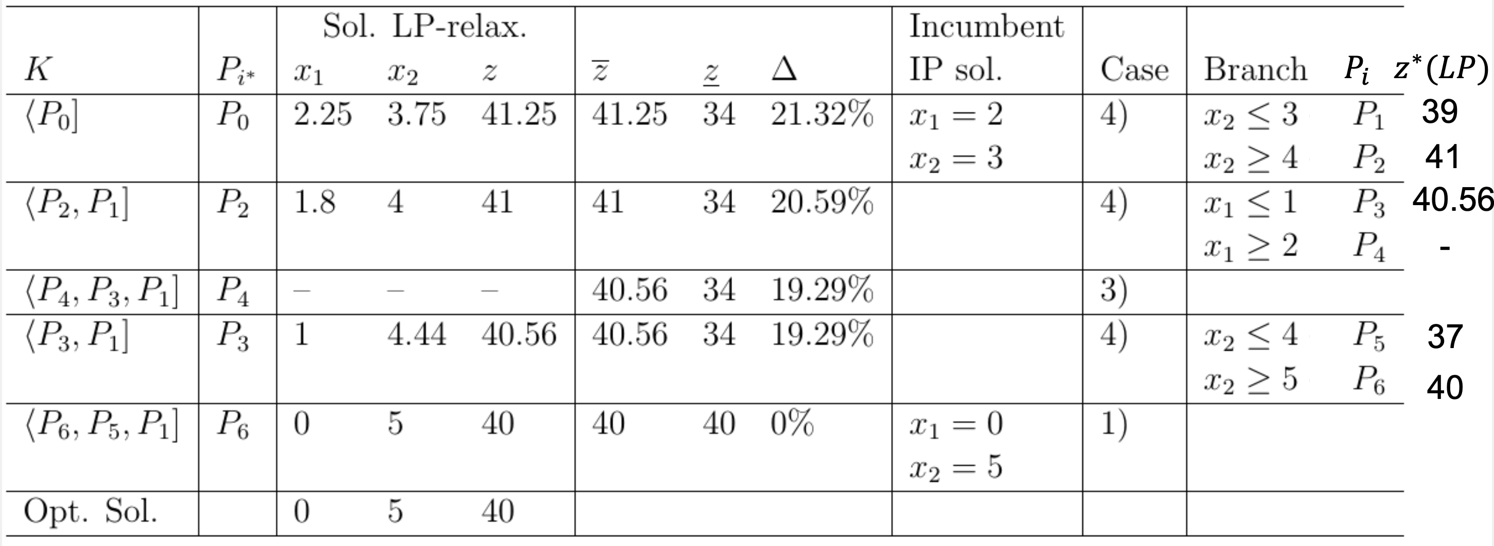
Table Format for Branch and Bound

The branch and bound process can be organized in a table format, tracking each subproblem’s details. The columns typically include:

• List of active nodes (subproblems to be solved) $K$
• Problem index $P_i$
• Solution of the relaxed problem $z^{\ast }(LP)$ (optimized variables in the selected node)
• Updated best bound, lower bound, and gap after solving the node
• Updated incumbent solution and best case so far
• Branching constraints made

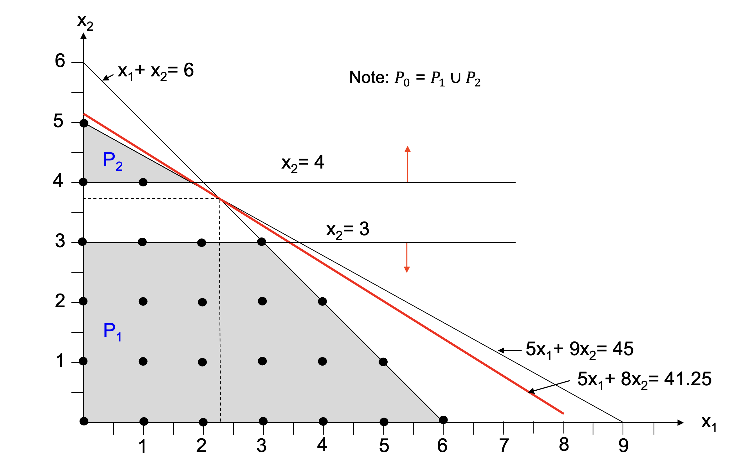
Branching

When the relaxed solution is not integer, branching is performed by selecting a variable with a fractional value and creating two new subproblems:

• Left Branch: Add a constraint that the variable must be $\le$ to its floor value.
• Right Branch: Add a constraint that the variable must be $\ge$ to its ceiling value.

In the lecture’s design, the number of the problem is its parent’s number + 1 for the left branch, and + 2 for the right branch: $p_0\to p_1$ (left) and $p_0\to p_2$ (right).

Variable Used for Branching

Most integer programs have multiple variables that need to be integer and can be branched on. A common strategy is to select the variable with the fractional value closest to 0.5, as this often leads to a more balanced search tree and can help in quickly finding feasible integer solutions. In the lecture, we arbitrarily choose $x_2$ if all (both) variables are fractional.

Candidate List:
Active nodes (branches to be considered) are tracked in a candidate list, here using LIFO for depth-first search. A node is removed from the list when it is solved using the LP relaxation. Depending on this solution, the node is discarded (if infeasible or suboptimal), kept as a candidate (if it yields a new best integer solution), or branched further into new subproblems added back to the list.

Selecting the Next Node

To select the next subproblem to solve from the candidate list, two strategies are commonly used:

• LIFO (Last In, First Out): Select the most recently added node, promoting depth-first search. This can quickly find feasible solutions but may not explore the most promising areas of the solution space first. LIFO is used in the lecture.
• Best-Bound: Select the node with the best upper bound (most promising solution). This strategy aims to explore the most promising areas of the solution space first, potentially leading to faster convergence to the optimal solution.

In case of ties, the node with the larger problem index is chosen next.

Solving the Subproblem

Solving each subproblem including the new constraint from scratch using the simplex is inefficient. Instead, the dual simplex method can be applied to re-optimize the solution after adding the new constraint.

Therefore, the new constraint is added to the final tableau of the parent problem. A new slack/surplus variable is created to account for the $\le$ or $\ge$ constraint, and its coefficient set to $1$. Then, Gaussian elimination is performed to set constrained variable to 0 in the new row. Finally, the dual simplex method is applied to re-optimize the tableau. See slide 26.

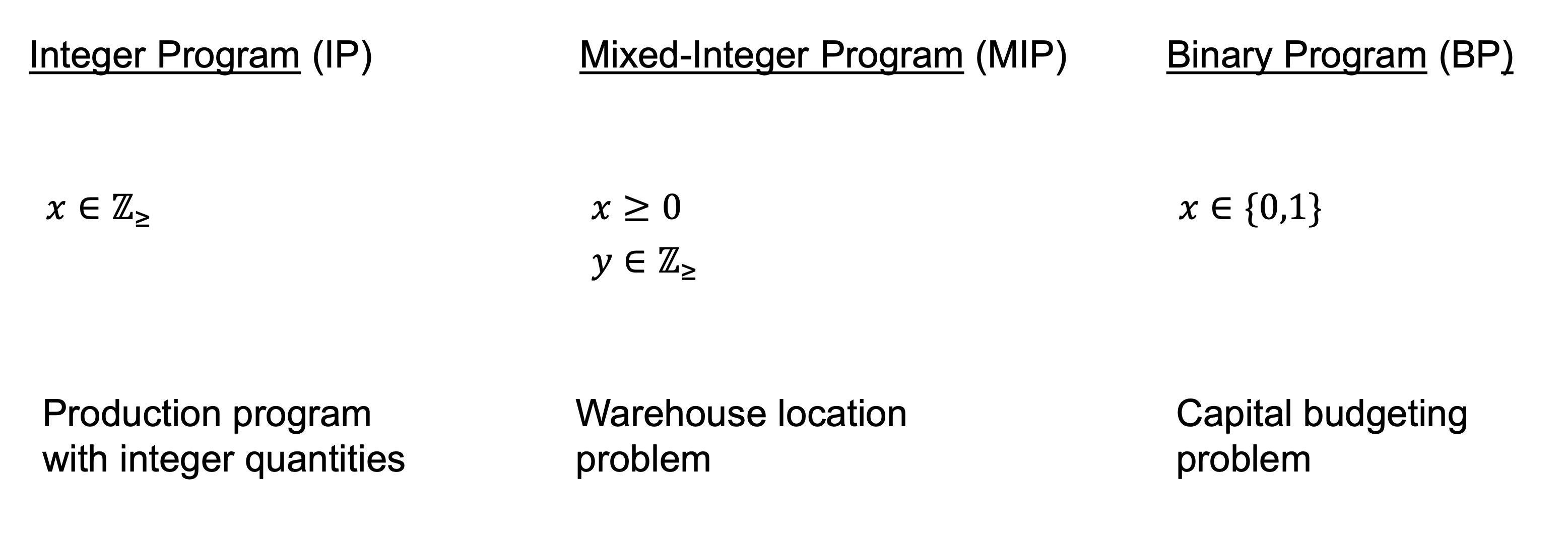
Binary Programs: Capital Budget Problem (CBP)

The Capital Budget Problem (CBP) is a specific type of integer programming problem that involves selecting a subset of investment projects to maximize the total net present value (NPV) while adhering to budget constraints. Each project has an associated cost and expected return, and the goal is to determine which projects to undertake given a limited budget. It involves:

• Binary Decisions: Each project can either be selected (1) or not selected (0).
• Budget Constraint: The total cost of selected projects must not exceed the available budget.

For CBP problems, we use the maximum upper bound node selection strategy to explore the most promising solutions first. At any time, at most one decision variable is fractional and can be used for branching.

Because of its binary nature, the CBP can be solved without the Simplex method, using only the branch and bound method.

Upper and Lower Bound in CBP

To determine UB and LB without Simplex solutions, we select projects in order of their profitability (NPV-to-cost ratio) until the budget is exhausted. The UB is calculated by including a fractional part of the next project that would exceed the budget, while the LB is determined by only including fully selected projects.

Branching in CBP

When branching in CBP, we select a project with a fractional decision variable and create two branches:

• Left Branch: Exclude the project (set decision variable to 0).
• Right Branch: Include the project (set decision variable to 1).

The added constraints (0 or 1) are then considered first in the upper/lower bound calculations for the subproblems, before considering projects by profitability.

If the constrained projects exceed the budget, the solution is of course infeasible. If the constrained projects exactly meet the budget, the solution is integer and can be used to update the incumbent solution.

Mixed-Integer Programming

A mixed-integer program is a linear program with integer and continuous variables. The branch and bound method can be applied similarly, but only the integer variables are considered for branching. The continuous variables are optimized using the simplex method at each node.

Mixed-integer programs were briefly demonstrated in the lecture using the warehouse location problem but not discussed further.