Decision Analysis

Material

• Slides
• Exercise Session 1, Session 2
• Recording Lecture 1

Choosing an Approach

Level of Uncertainty

• Certain: Deterministic future - known state and outcome. (p. 5)
• Uncertain: Multiple possible futures with unknown probabilities.
• Risk: Multiple possible futures with known probabilities, all outcomes known.

Decision Context

• Single Goal vs. Multiple Goals (criteria) (p. 6)
• Single Decision Maker vs. Multiple Decision Makers (p. 7)
• Static (one-shot) vs. Dynamic (multi-stage over time) (p. 8)
• Opponents: Nature (passive) vs. Other Decision Makers (active antagonists) (p. 9)
• Types of Problems: Optimization vs. Game Theory

Decisions Under Uncertainty: Decision Matrix

• Context: Uncertainty, Single Goal, Single DM, Static, Game against Nature. (p. 11)
• One of m alternative actions is chosen ($a_1,...,a_m$).
• One of n scenarios will take place ($s_1,...,s_n$).
• Sequence: Action $a_i$ → Scenario $s_j$ → Outcome $e_{i,j}$. (p. 14)
• The outcome $e_{i,j}$ is evaluated by a payoff function $v(e_{i,j})$, resulting in a payoff matrix.
• An alternative $a_i$ is efficient (non-dominated) if no other alternative $a_k$ exists that is better in at least one scenario and not worse in any other. (p. 19)
• Example: The Newsvendor Problem demonstrates how to build and reduce a decision matrix. (p. 15)

Decision Rules

• There is no single optimal rule; the choice reflects the decision maker’s attitude towards risk.

Risk-Averse and Risk-Seeking

• Risk-Averse: Prefers a certain outcome over a gamble with a higher or equal expected value.
• Risk-Seeking: Prefers a gamble over a certain outcome, even if the expected value is lower.
• Entrepreneurs often tend to be risk-seeking.

$i\star =\arg \dots$ denotes the index of the argument for which the statement is true.

Maximin: Wald Rule

Chooses the alternative with the best worst-case outcome.

• For pessimistic, risk-averse decision-makers.
• First, find the minimum outcome for each alternative: ${\underline{e}}_i={\min }_{j=1}^n\{e_{i,j}\}$.
• Then, choose the alternative with the maximum of these minimums: $i^{\star }=\arg {\max }_{i=1}^m\{{\underline{e}}_i\}$. (p. 22)

Maximax

Chooses the alternative with the best possible outcome.

• For optimistic, risk-seeking decision-makers.
• First, find the maximum outcome for each alternative: ${\overline{e}}_i={\max }_{j=1}^n\{e_{i,j}\}$.
• Then, choose the alternative with the maximum of these maximums: $i^{\star }=\arg {\max }_{i=1}^m\{{\overline{e}}_i\}$. (p. 23)

Hurwicz

A compromise between Maximin and Maximax, using an optimism parameter $\lambda \in [0,1]$.

• $\lambda =1$ is equivalent to Maximax, $\lambda =0$ is equivalent to Maximin.
• A weighted average is calculated for each alternative: $H_i(\lambda )=\lambda \cdot {\max }_j\{e_{ij}\}+(1-\lambda )\cdot {\min }_j\{e_{ij}\}$.
• Choose the alternative with the highest weighted average: $i^{\star }=\arg {\max }_{i=1}^m\{H_i(\lambda )\}$. (p. 24)
• The optimal choice can be visualized as a function of $\lambda$. (p. 25)

Minimax Regret Rule

Chooses the alternative that minimizes the maximum possible regret.

• Regret (or opportunity loss) is the difference between the best possible outcome for a given scenario and the actual outcome of the chosen alternative. (p. 26)
• First, construct a regret matrix: $r_{i,j}=({\max }_k\{e_{k,j}\})-e_{i,j}$.
• Then, apply the Minimax principle to the regret matrix: find the maximum regret for each action (${\overline{r}}_i={\max }_j\{r_{i,j}\}$) and choose the action with the minimum of these maximums ($i^{\star }=\arg {\min }_i\{{\overline{r}}_i\}$). (p. 28)

Laplace

Chooses the alternative with the highest average outcome (if equally likely).

• Assumes that all scenarios are equally likely.
• Calculate the average outcome for each alternative.
• Choose the alternative with the highest average outcome: $i^{\star }=\arg {\max }_{i=1}^m\left\{\frac{1}{n}{\sum }_{j=1}^n{e}_{i,j}\right\}$. (p. 29)

Decisions Under Risk: Expected Utility Theory

• Context: Risk, Single Goal, Single DM, Static, Game against Nature. (p. 30)
• Each scenario $s_j$ has a known probability $p_j$, with ${\sum }_{j=1}^n{p}_j=1$.

St. Petersburg Lottery

• A hypothetical lottery where a coin is tossed until it lands on tails. If tails appears on the $n$-th toss, the payoff is $2^n$.
• The expected value is infinite: $E={\sum }_{n=1}^{\infty }{\left(\frac{1}{2}\right)}^n\cdot 2^n={\sum }_{n=1}^{\infty }1=\infty$.
• However, most people would only pay a small, finite amount to play, demonstrating that expected value alone is not a sufficient criterion for decisions. This is known as the St. Petersburg Paradox. (p. 31)

Expected Value & Utility (Bernoulli)

A utility function $u(e)$ is needed to map outcomes to the decision maker’s subjective utility.

• Expected Value of a lottery $L_i$: $E(L_i)={\sum }_{j=1}^n{p}_j\cdot e_{i,j}$
• Expected Utility of a lottery $L_i$: $EU(L_i)={\sum }_{j=1}^n{p}_j\cdot u(e_{i,j})$

Where $p_j$ is the probability of scenario $s_j$.

Certainty Equivalent (CE)

The guaranteed amount of money that a decision maker would find equally desirable to a given lottery.

It is the value for which the utility of the certain amount equals the expected utility of the lottery: $u(CE)=EU(L)$. (p. 36)

Risk Premium (RP)

The difference between the expected value of a lottery and its certainty equivalent.

• $RP(L_i)=E(L_i)-CE(L_i)$. (p. 37)
• It represents the amount an individual is willing to forgo to avoid the risk of the lottery. (ai)
• Risk-Averse: $RP>0$
• Risk-Seeking: $RP<0$
• Risk-Neutral: $RP=0$

Utility Function $u(e)$

• Scaling: The utility function is typically scaled by setting the utility of the worst outcome $e^{-}$ to 0 and the best outcome $e^{+}$ to 1. $u(e^{-})=0$, $u(e^{+})=1$. (p. 51)
• Ordering: If outcome $e_1$ is preferred to $e_2$, then $u(e_1)>u(e_2)$.
• Risk Attitude:
  • Risk-Averse: Concave function ($u^{\prime \prime }(e)<0$). The marginal utility of money decreases.
  • Risk-Seeking: Convex function ($u^{\prime \prime }(e)>0$). The marginal utility of money increases.
  • Risk-Neutral: Linear function ($u^{\prime \prime }(e)=0$).
• Empirically, decision makers can exhibit mixed risk attitudes — risk-avoidant or seeking at different values. (p. 46)

Arrow-Pratt Measure of Absolute Risk Aversion

Determines the local risk attitude of a decision maker at outcome level x:
$AP(x)=-\frac{u^{\prime \prime }(x)}{u^{\prime }(x)}$

• $AP(x)>0$: risk-averse
• $AP(x)<0$: risk-seeking
• $AP(x)=0$: risk-neutral

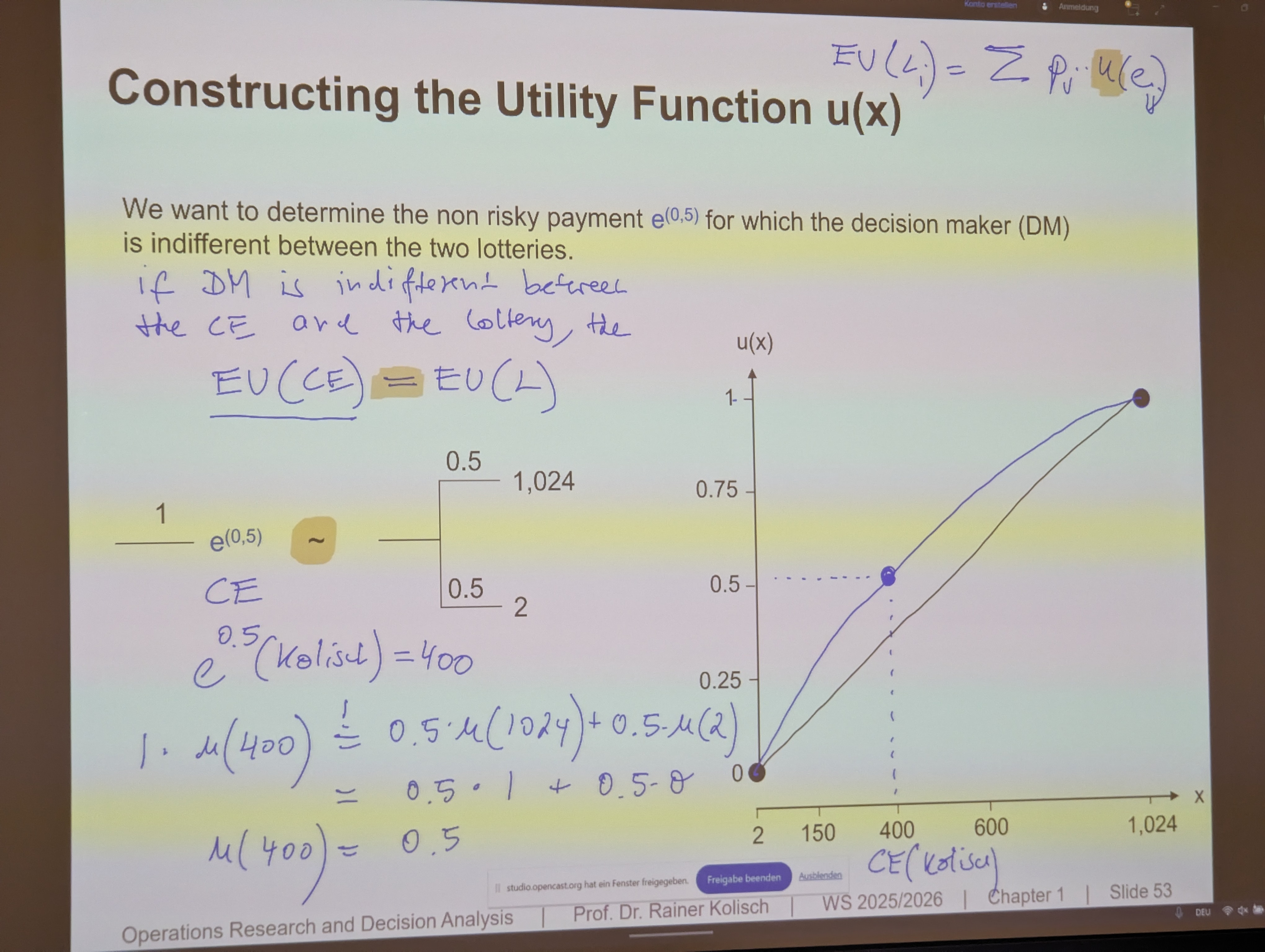
Constructing The Utility Function

• The utility function is constructed by finding certainty equivalents for different lotteries.
• If a Decision Maker (DM) is indifferent between a certain payment (CE) and a lottery (L), their utilities must be equal: $u(CE)=EU(L)$.
• Procedure: (p. 53)
  1. Define the best ($e^{+}$) and worst ($e^{-}$) possible outcomes and scale the utility function, e.g., $u(e^{+})=1$ and $u(e^{-})=0$.
  2. Consider a simple lottery, e.g., a 50/50 chance of winning $e^{+}$ or $e^{-}$. The expected utility is $EU(L)=0.5\cdot u(e^{+})+0.5\cdot u(e^{-})=0.5$.
  3. Ask the DM for their certainty equivalent (CE) for this lottery. This CE gives a point on their utility curve: $(CE,0.5)$.
  4. Repeat this process with different probabilities and outcomes to plot more points and elicit the shape of the utility function.
• Example: For a lottery with a 50% chance of 1024 and 50% of 2, we set $u(1024)=1$ and $u(2)=0$. The $EU(L)=0.5$. If the DM’s CE is 400, then we have the point $u(400)=0.5$.

Photo

$\mu -\sigma$ Representation

An alternative’s risk profile can be characterized by its expected value ($\mu$) and its standard deviation ($\sigma$).

• Expected Outcome ($\mu$): $\mu (a_i)={\sum }_{j=1}^n{p}_j\cdot e_{i,j}$
• Variance (${\sigma }^2$): ${\sigma }^2(a_i)={\sum }_{j=1}^n{p}_j\cdot (e_{i,j}-\mu (a_i){)}^2$
• Standard Deviation ($\sigma$): $\sigma (a_i)=\sqrt{{\sigma }^2(a_i)}$
• The decision maker’s preference can be visualized with indifference curves in a $\mu -\sigma$ diagram. Each curve connects points ($\sigma ,\mu$) that provide the same level of utility. (p. 59)
  • Risk-Averse: Prefers higher $\mu$ and lower $\sigma$. Indifference curves are upward sloping.
  • Risk-Seeking: Prefers higher $\mu$ and higher $\sigma$. Indifference curves are downward sloping.
  • Risk-Neutral: Prefers higher $\mu$ and is indifferent to $\sigma$. Indifference curves are horizontal.

Preference Function $\Phi (\mu ,\sigma )$

The preference function, $\Phi (a_i)=f(\mu (a_i),\sigma (a_i))$, formalizes the decision maker’s trade-off between expected return ($\mu$) and risk ($\sigma$). (p. 72)

• Risk-Neutral: The DM only considers the expected value. $\Phi (a_i)=\mu (a_i)$ (p. 73)
• Risk-Seeking: The DM values higher variance. Example: $\Phi (a_i)=\mu (a_i)+0.5\cdot {\sigma }^2(a_i)$ (p. 74)
• Risk-Averse: The DM penalizes variance. Example: $\Phi (a_i)=1.5\cdot \mu (a_i)-2\cdot \sigma (a_i)$ (p. 75)

Drawbacks of the $\mu -\sigma$ Rule:

• It does not provide guidance on how to calibrate the preference function $\Phi$.
• It cannot determine the risk attitude of the decision maker on its own. (p. 76)# Decision Trees

Decision Trees

• Context: Risk, Single Goal, Single DM, Dynamic, Game against Nature. (p. 78)
• Used for multi-stage decision problems where decisions and chance events unfold over time.

Nodes

• ◻️ Decision Nodes: The DM chooses an action.
• ⚪ Chance Nodes: A scenario occurs with a certain probability.
• ◀︎ End Nodes: Represent the final outcome.

Solving Decision Trees

Rollback Procedure

• Start from the end nodes and work backward to the root.
• At chance nodes, calculate the expected utility (or value) of the subsequent branches.
• At decision nodes, choose the action that leads to the branch with the highest expected utility.
• The process determines the optimal policy (a complete plan of which action to take at every decision node). (p. 81)
• Example: See (p. 82)

Test Markets

• A practical application of decision trees to assess the value of information.
• A decision is made whether to launch a product directly, conduct a test market first, or not launch at all.
• The test market provides imperfect information (e.g., a “positive” or “negative” signal) that is used to update the probabilities of the actual market being a success or failure (using Bayes’ theorem). (ai)
• By comparing the expected utility of launching with a test market versus without, one can determine the value of the test market information. (p. 87)

Value of Perfect Information (VPI)

• The VPI is the maximum amount a decision maker would be willing to pay for perfect information about the future.
• It is calculated as the difference between the expected value with perfect information (EVwPI) and the expected value without perfect information (EVwoPI).
• EVwPI: The expected value if the decision maker could know the outcome of the chance event before making their decision. To calculate it, you reverse the order of decision and chance nodes and choose the best action for each scenario. (p. 91)
• EVwoPI: The expected value of the best action without having the perfect information (this is the standard outcome of solving the decision tree).
• $VPI=EVwPI-EVwoPI$
• The VPI provides an upper bound on how much to spend on gathering information. (ai)

Scoring Model: Multi-Criteria

• Context: Deterministic, Multiple Goals, Single DM, Static. (p. 99)
• The Scoring Model evaluates alternatives by combining their performance across multiple criteria into a single score.
• Other models for multi-criteria decisions include the Analytical Hierarchy Process (AHP) and Multi-Attribute Utility Theory (MAUT).

Process

After determining objectives:

1. Determine Criteria Weights ($w_j$)

   • Assign an importance value $g_j$ to each criterion $j$ (e.g., on a scale from 1 to 5).
   • Calculate the normalized weight for each criterion: $w_j=\frac{g_j}{{\sum }_k{g}_k}$. (p. 102)

2. Define Value Functions ($v_j$)

   • For each criterion, define a value function $v_j(e_{i,j})$ that maps all possible outcomes $e_{i,j}$ (from a utility function) for an alternative $a_i$ to a normalized scale of [0, 1].
   • The function must be monotonic, the best outcome receives a value of 1, the worst 0.
   • Example: For a “cost” criterion, the lowest cost gets 1 and the highest gets 0. For a “success” criterion, the highest success gets 1 and the lowest gets 0. (p. 107)
   • If outcomes are qualitative (e.g., “low”, “good”), they must first be converted to a quantitative scale. (p. 103)

3. Calculate Overall Score ($S(a_i)$)

   • The overall score for each alternative is the weighted sum of its normalized values across all criteria.
   • $S(a_i)={\sum }_j{w}_j\cdot v_j(e_{i,j})$
   • The alternative with the highest score is chosen. (p. 108)

Sensitivity Analysis

• After calculating the scores, a sensitivity analysis can be performed to check how robust the result is with respect to the criteria weights.
• This involves analyzing how the final scores and the optimal choice change as the weights ($w_j$) are varied. (p. 110)