Conjoint Analysis – Understanding Preferences

Resources

• Slides: Conjoint Analysis
• Exercises: Conjoint Analysis
• Recordings: Conjoint Analysis

Conjoint Analysis

Conjoint analysis is a statistical technique used to understand how consumers value different attributes of a product or service. It helps identify the optimal combination of features that maximizes consumer preference. It assumes that preferences are a combination of all attributes: considered jointly. It is often considered an extension of Regression Analysis — Model Fitting, because regression is used to estimate the part-worth utilities of each attribute level.

This is useful for simulating the preference impact of new products, changes to products, pricing strategies, or discounting products.

Steps in Conjoint Analysis

1. Identify Attributes & Levels: Determine the key attributes of the product/service and their respective levels. For example, for a smartphone, attributes could be battery life (8 hours, 12 hours, 16 hours), camera quality (12 MP, 48 MP), and price ($500,$700, $900).
2. Design the Study: Create a set of hypothetical product profiles by combining different levels of attributes. This can be done using full-profile or fractional factorial designs.
3. Collect Data: Present the profiles to respondents and ask them to rank, rate, or choose between different options. This data will be used to estimate the part-worth utilities.
4. Estimate Part-Worth Utilities: Use regression analysis to estimate the part-worth utilities for each attribute level based on the collected data. These utilities represent the value that consumers assign to each level of an attribute.
5. Analyze Results: Analyze the estimated utilities to determine the relative importance of each attribute and identify the optimal product configuration.

Selecting Attributes

When selecting attributes for conjoint analysis, consider the following criteria:

• Relevance: Attributes must be relevant for people’s preferences
• Actionability: Attributes should be actionable for decision-making
• Realistic & Feasible: The attribute levels and their combinations have to be plausible
• Number of Attributes: Limit the number of attributes to avoid overwhelming respondents (typically 5-7 attributes)
• Compensatory vs. Non-Compensatory: Attributes should able to compensate for each other (e.g., a higher price can be compensated by better quality); the attribute levels should not be exclusion cirteria
• Independence: Attributes should be independent of each other to avoid confounding effects

Designing the Options

In a full profile design, attributes are orthogonal (uncorrelated), and all possible combinations of attribute levels are presented to respondents. However, this can lead to a large number of profiles, which may be impractical. There are alternative designs:

Fractional Orthogonal Designs

Fractional orthogonal designs present a subset of all possible profiles while maintaining orthogonality. This reduces the number of profiles respondents need to evaluate, making the study more manageable.
Such a design can be created, for example, using a simulation in R using the conjoint package.

Collecting Preference Data

Preference data can be collected using various ordinal (rankings) or metric (ratings) methods:

Ordinal Methods

• Ranking: Respondents rank the profiles from most to least preferred.
• Paired Comparisons: Respondents choose between pairs of profiles.

Metric Methods

• Rating Scales: Respondents rate each profile on a scale (e.g., 1 to 10).
• Dollar Value: Respondents indicate how much they would be willing to pay for each profile.
• Constant Sum: Respondents allocate a fixed number of points across profiles based on their preferences.

Analyzing The Data

Part-worth utilities can be estimated using regression analysis. The structure of a conjoint analysis model is similar to that of a multiple regression model:

$$u_k=b_0+\sum _{j=1}^J{X}_{jk}\times B_j$$

The latent utility $u_k$ for profile $k$ is modeled as a function of the attribute levels $X_{jk}$ and their corresponding coefficients (part-worth utilities) $B_j$. The intercept $b_0$ represents the baseline utility.

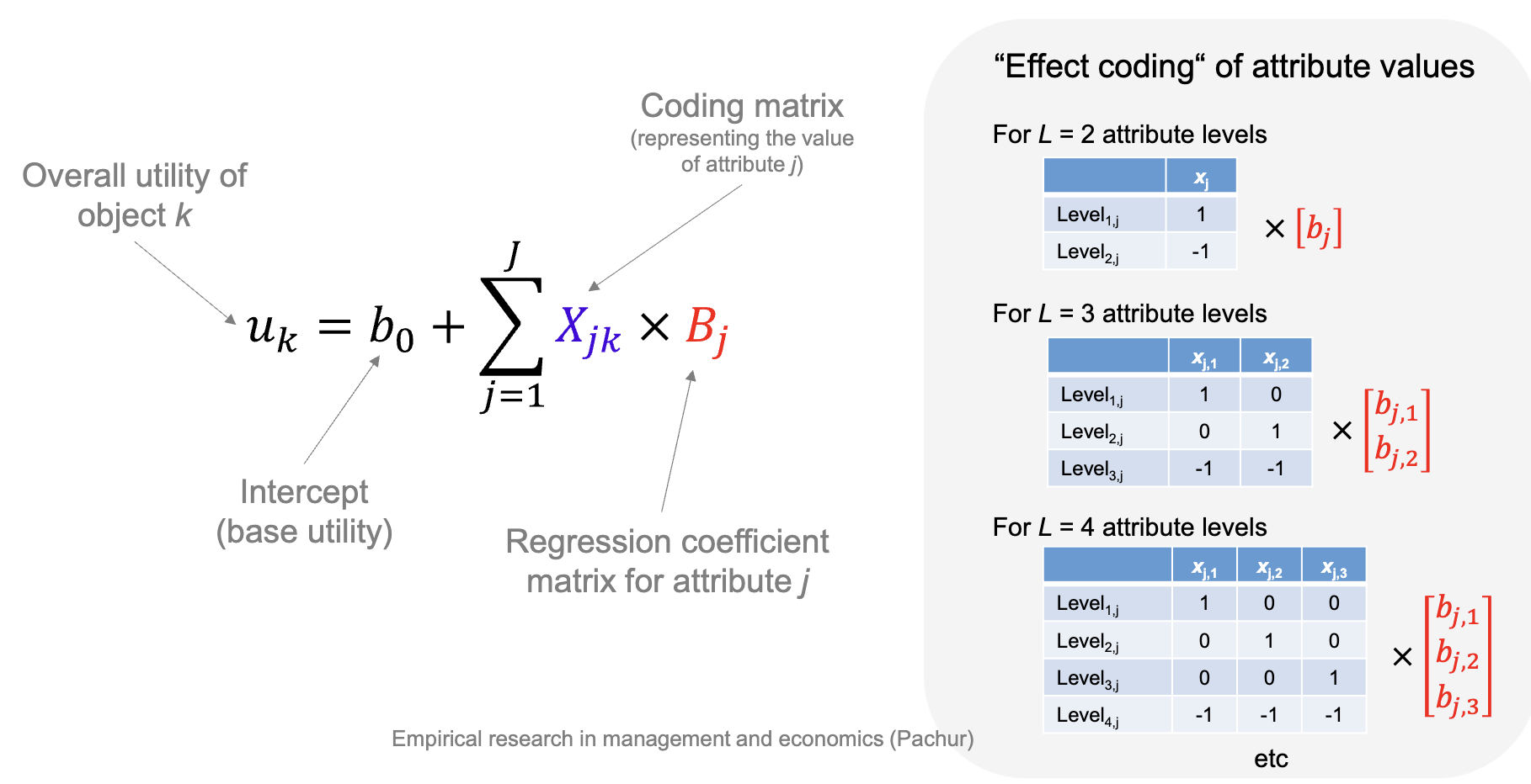
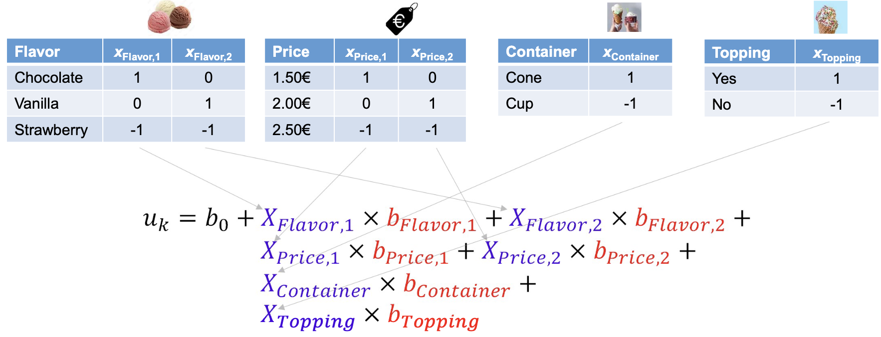
The coding matrix $X$ represents the attribute levels for each profile. Effect coding is commonly used, where each attribute level is represented by a binary (1 or 0) regression weight, and one level is omitted as the reference category. An alternative is dummy coding.

The utility of each profile is the sum of the part-worth utilities of its attribute levels. The estimated coefficients from the regression represent the part-worth utilities for each attribute level:

$$u_k=X_{\text{attribute 1, level 1}}\times B_{\text{attribute 1, level 1}}+X_{\text{attribute 1, level 2}}\times B_{\text{attribute 1, level 2}}+X_{\text{attribute 2}}\times B_{\text{attribute 2}}+...$$

Partworth Utilities

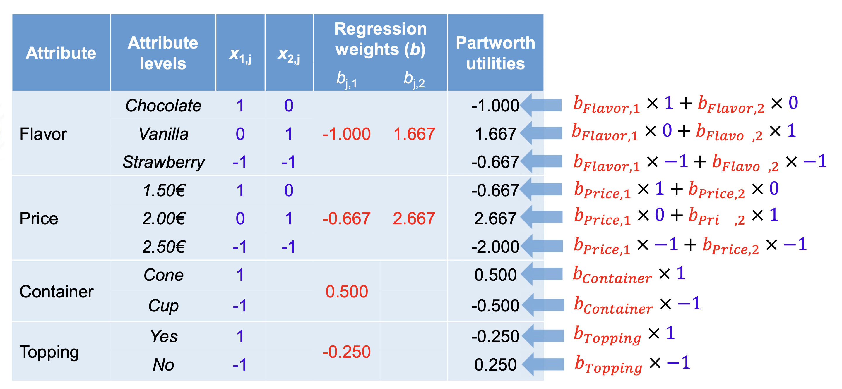
Based on the regression results, part-worth utilities can be calculated for each attribute level. These utilities indicate the relative preference for each level of an attribute.

• Positive utilities indicate a preference for that level, while negative utilities indicate a dislike.
• The magnitude of the utility indicates the strength of the preference.
• They are often graphed as bar charts for better visualization.

Partworth utilites are calculated by multiplying the respective regression coefficient matrix row with the attribute level coding.

All part-worth utilities for an attribute sum to zero, if effect coding is used.

Attribute Importance

The importance of each attribute can be calculated by examining the range of part-worth utilities for that attribute. The importance score for an attribute is given by:

$w_j=\frac{\underset{l}{\max }\{p_{jl}\}-\underset{l}{\min }\{p_{jl}\}}{\sum _{j=1}^J(\underset{l}{\max }\{p_{jl}\}-\underset{l}{\min }\{p_{jl}\})}$

In other words, the difference between the highest and lowest part-worth utility for an attribute is divided by the sum of such differences across all attributes. This yields a relative importance score for each attribute, indicating how much it influences overall preference compared to other attributes.

Importance scores for all attributes sum to 1.

Estimating Utility of Options

Once part-worth utilities are estimated, the overall utility of any product profile can be calculated by summing the part-worth utilities of its attribute levels:

$$u_k=b_0+\sum _{j=1}^J{X}_{jk}\times B_{jl}$$

Example on slide 25.

Predicting Utility of New Profiles

In the same way as predicting the utility of existing profiles, the utility of new product profiles can be predicted by summing the part-worth utilities of their attribute levels. This allows for simulating consumer preferences for hypothetical products that were not part of the original study.