Resources
- Slides: Simple Regression, Multiple Regression, Logit
- Exercises: Simple Regression, Multiple Regression, Logit
- Recordings: Simple Regression (Transcript), none for Multiple Regression, Logit
Regressions describe the relationship between a dependent variable (outcome) and one or more independent variables (predictors). They are widely used in empirical research to analyze data and make predictions.
Mean-Centering
By subtracting the population mean from each value of a predictor variable, centering helps make the y-intercept more interpretable in regression models. The intercept then represents the expected value of the dependent variable when all independent variables are at their average values.
Coefficient of Determination
measures the percentage share of variance in the dependent variable that can be explained by the independent variables in a regression model.
For a single predictor and outcome, it’s the square of a the Pearson correlation coefficient .It’s simply the proportion of model variation to total variation:
The adjusted accounts for the number of predictors in the model, penalizing for adding variables that do not improve the model fit (sample size N, predictor count k):
Confidence Interval
The confidence interval provides a range of values within which we can be confident that the true population parameter (e.g., mean, proportion) lies, based on our sample data. It reflects the uncertainty associated with estimating the parameter from a sample.
The formula for a confidence interval for a mean is:
Prediction Interval
A prediction interval provides a range of values within which we can expect a new individual observation to fall, given a certain level of confidence. It accounts for both the uncertainty in estimating the population parameter and the variability of individual observations around that parameter.
The formula for a prediction interval is:
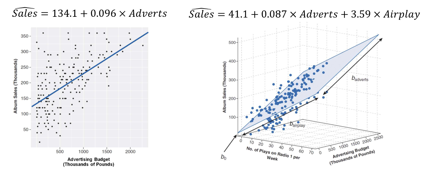
Simple Regression
Simple regression involves one dependent variable and one independent variable. For simple linear regressions, the goal is to fit a linear model to these two variables.
A simple line fitted to the data, with a slope and an intercept determining the predicted value.
As clear from the formula, has to be significantly different from 0 to claim a relationship between X and Y.
This assumes:
- Linearity: The relationship between X and Y is linear.
- Homoscedasticity: The variance of residuals is constant across all levels of X.
- Normal Distribution
Ordinary Least Squares (OLS)
A method to estimate the parameters of a linear regression model by minimizing the sum of squared differences between observed and predicted values. OLS is a simple and widely used technique for fitting linear models, however, it assumes linearity and is sensitive to outliers.
OLS can be solved algebraically, formulas on p. 13, but not relevant for the exam.
Confidence Interval
Formula for the confidence interval of a predicted mean response in a simple linear regression:
Prediction Interval
Formula for the precision of a single predicted value in a simple linear regression:
Evaluating Fit: t-test on
To evaluate whether the slope is significantly different from 0, we can use a t-test. The t-statistic is calculated as:
Where is the standard error of the slope estimate. The degrees of freedom (df) for this test is , where is the number of observations and the number of predictors:
Checking for Linearity
Three approaches are used to check whether the relationship between the independent and dependent variable is linear.
Visual Inspection for Linearity
When looking at a scatterplot of predictor and outcome, the points should roughly follow a straight line. The average value of residuals should be similar across the predictor values.
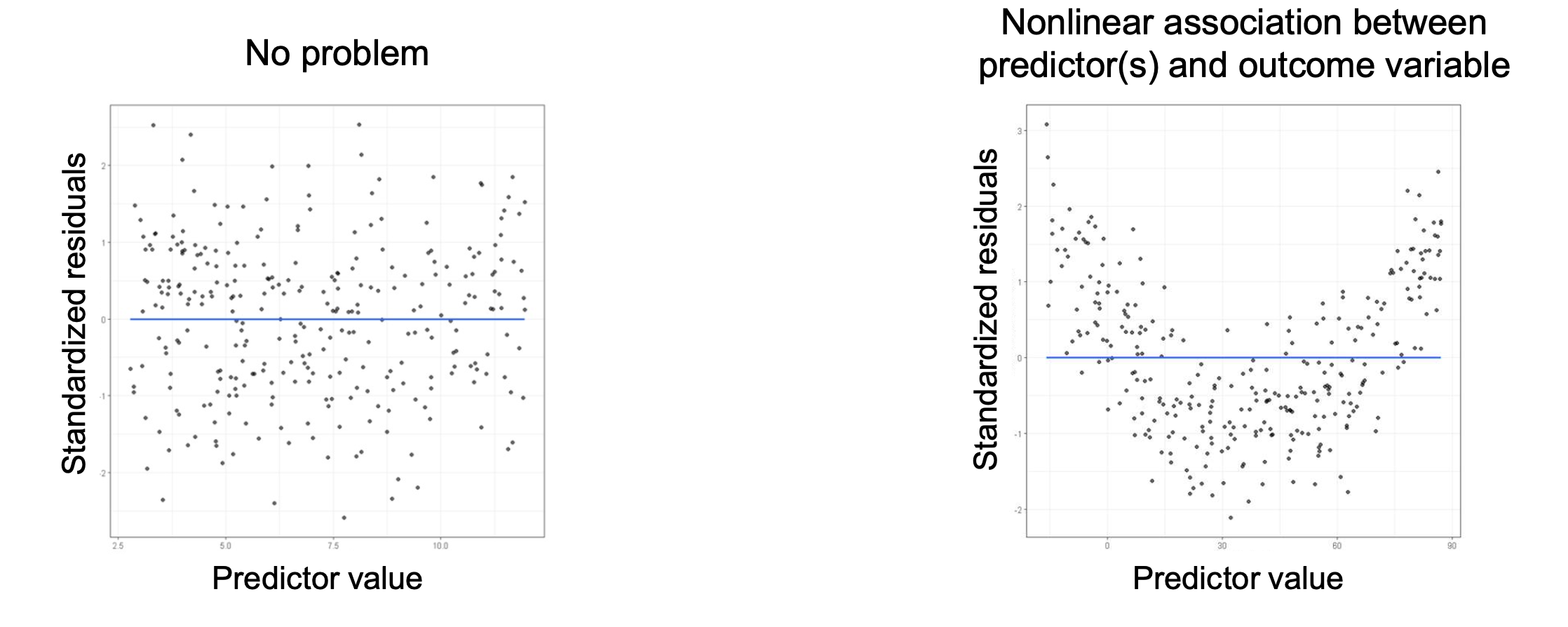
Residual Analysis
When plotting the residuals against the predicted values, there should be no discernible pattern. If a pattern is detected, it indicates a non-linear relationship.
Transformations
If a non-linear relationship is detected, transformations such as logarithmic or polynomial transformations might be applicable to the data to achieve linearity. The transformed model can then be evaluated for linearity again.
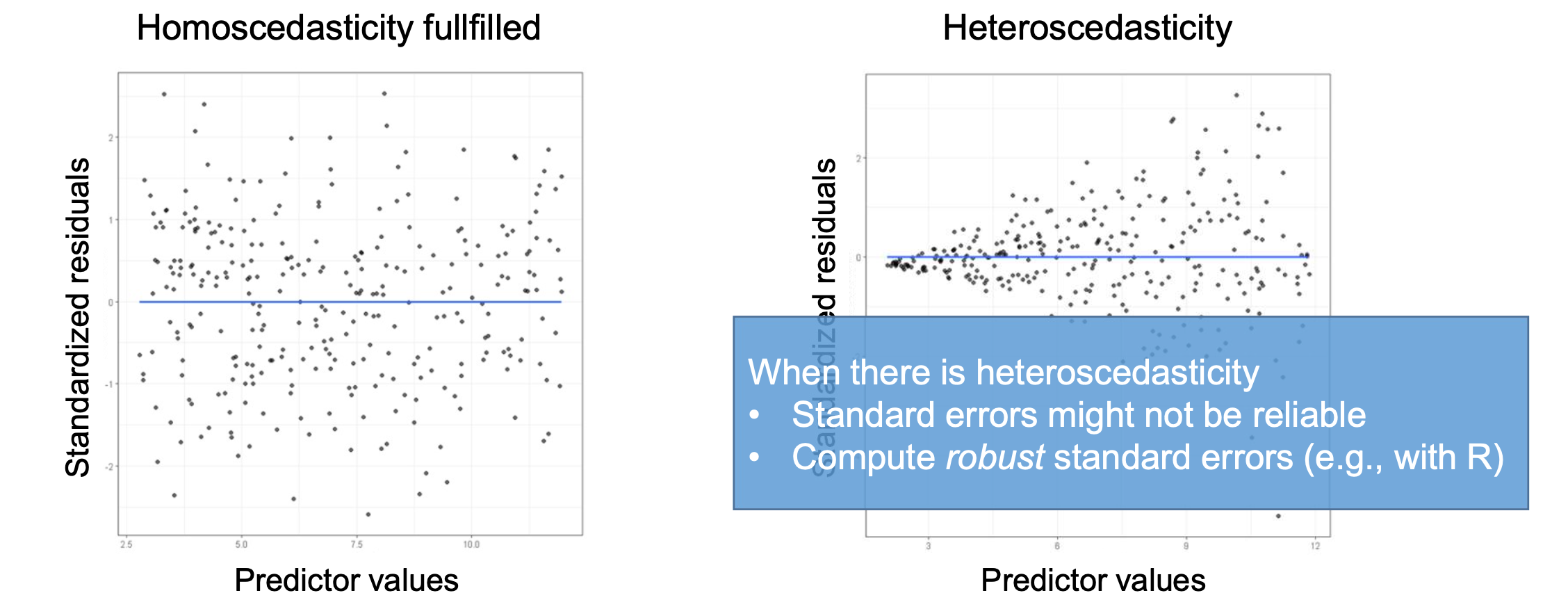
Checking for Homoscedasticity
Homoscedasticity means that the variance of the residuals is constant across all levels of the independent variable.
This can also be checked using a visual inspection of residuals: If the spread of residuals is roughly constant across all predicted values, homoscedasticity is present. If the spread increases or decreases with predicted values, heteroscedasticity is indicated.
To account for heteroscedasticity, robust standard errors can be used in the regression analysis.
Checking for Normal Distribution
Normality of residuals can be checked using a Q-Q plot, where the quantiles of the residuals are plotted against the quantiles of a normal distribution. If the points fall approximately along a straight line, the residuals are normally distributed.
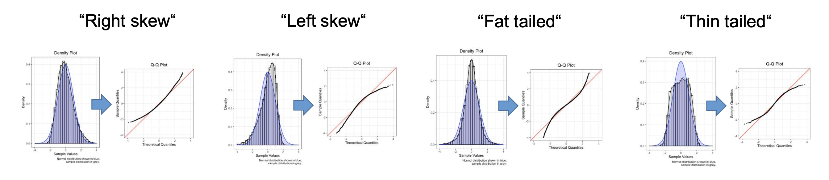
Q-Q Plot
Quantile-Quantile plots visualize how the distribution of a dataset compares to a theoretical distribution, such as the normal distribution.
On the x-axis, the expected quantile values of the theoretical distribution are plotted, while on the y-axis, the quantiles of the observed data are plotted.
Multiple Regression
Multiple regression involves multiple independent variables (predictors) predicting a single dependent variable (outcome). The goal is to understand the relationship between several predictors and the outcome.
A plane (or hyperplane in higher dimensions) fitted to the data, with coefficients and an intercept determining the predicted value:
In addition to the Simple Linear Regression assumptions of linearity, homoscedasticity, and normal distribution, multiple regression assumes:
- No Multicollinearity: The independent variables should not be highly correlated with each other. High multicollinearity can make it difficult to determine the individual effect of each predictor on the dependent variable.
Determining Sample Size
Additional predictors require larger sample sizes to maintain statistical power. A common rule of thumb is to have at least 10-15 observations per predictor variable. A power analysis (through G*Power) can provide a more precise estimate based on the expected effect size, significance level, and desired power.
Checking for Multicollinearity
Two approaches are used to identify multicollinearity between independent variables.
If there is multicollinearity, consider dropping redundant predictors or combining highly correlated variables into a single composite variable using Factor Analysis techniques like PCA.
Correlation Matrix
A correlation matrix displays the pairwise correlations between all independent variables. High correlations (e.g., above 0.8 or below -0.8) indicate potential multicollinearity issues.
Variance Inflation Factor (VIF)
The VIF quantifies how much the variance of a regression coefficient is increased due to multicollinearity. It’s the inverse of the tolerance, which measures the proportion of variance in an independent variable that is not explained by other independent variables.
Where is the coefficient of determination obtained by regressing the -th independent variable against all other independent variables. A VIF value greater than 10 is often considered indicative of significant multicollinearity, and the average VIF across all predictors should not substantially exceed 1.
Standardized Regression Coefficients
Standardized regression coefficients (beta weights) allow for the comparison of the relative importance of each predictor variable in the model: They describe the change in the dependent variable in standard deviations for a one standard deviation change in the predictor variable. These coefficients are determined by converting dependent and independent variables to z-scores, with a mean of 0 and a standard deviation of 1.
Evaluating Fit: F-test
To evaluate the overall fit of the multiple regression model, an F-test is used. This tests if the model explains significantly more variance than a model without any predictors. The F-statistic is calculated as:
This is then compared to a critical value from the F-distribution with and degrees of freedom.
Evaluating Individual Predictors: t-test on
To evaluate whether each coefficient is significantly different from 0, we can use a t-test. The t-statistic for each predictor is calculated in the same way as in simple regression:
If the calculated t-statistic exceeds the critical value from the t-distribution with degrees of freedom, the predictor significantly contributes to the model.
Moderation Analysis
To identify moderator variables that influence the strength or direction of the relationship between an independent variable and a dependent variable, interaction terms are included in the regression model. An interaction term is created by multiplying the independent variable with the moderator variable:
If the coefficient of the interaction term () is significantly different from 0, it indicates that the moderator variable influences the relationship between the independent and dependent variables.
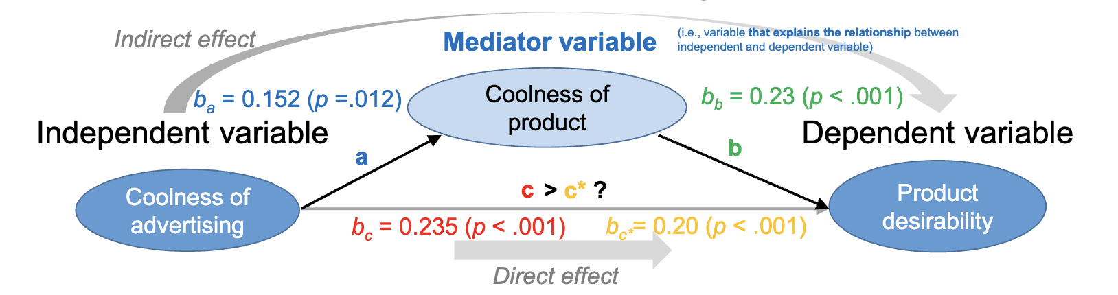
Mediation Analysis
Mediation analysis examines whether the effect of an independent variable on a dependent variable is transmitted through a mediator variable. This requires three conditions:
- The relationship between independent and dependent variable is significant.
- The relationship between independent variable and mediator is significant.
- The relationship between mediator and dependent variable (controlling for independent variable) is significant, and the direct effect of independent variable on dependent variable is reduced when the mediator is included.
To test this, three regression models are estimated:
- Regress the dependent variable on the independent variable:
- Regress the mediator on the independent variable:
- Regress the dependent variable on both the independent variable and the mediator:
In the bootstrap approach used in class, the indirect effect is calculated as the product of the coefficients from the second and third models: . A confidence interval for this indirect effect is generated through resampling. If the confidence interval does not include 0, it indicates a significant mediation effect.
An alternative is the Sobel test.
Encoding Categorical Variables
To work with categorical independent variables in regression analysis, dummy coding is used. This involves creating binary (0/1) variables for each category of the categorical variable, except for one reference category. For example, for a categorical variable with three categories (A, B, C), two dummy variables would be created:
| Category | Dummy 1 (B) | Dummy 2 (C) |
|---|---|---|
| A | 1 | 0 |
| B | 0 | 1 |
| C | 0 | 0 |
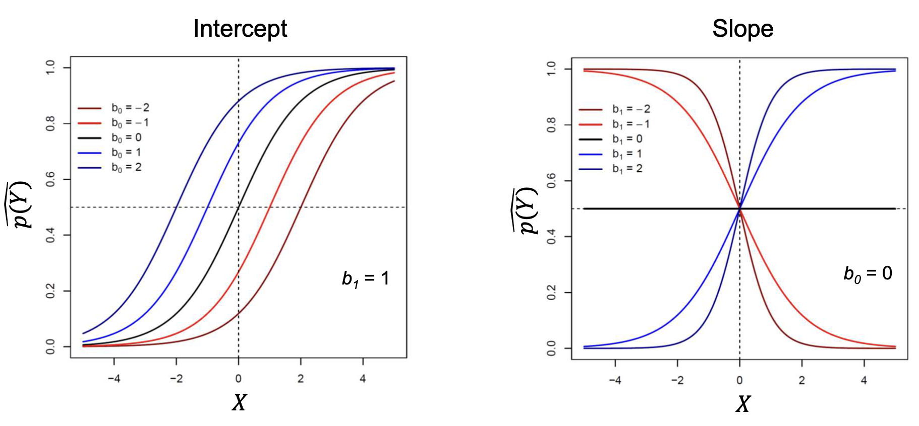
Logistic Regression
Logistic regression is used when the dependent variable (outcome) is categorical. It models the probability of the occurrence of an event by fitting data to a logistic function. It can be fitted to one or more independent variables.
It’s defined as the inverse of the logit function, which is the natural logarithm of the odds of the event occurring.
The coefficients are estimated using Maximum Likelihood Estimation (MLE), which finds the parameter values that maximize the likelihood of observing the given data.
Logistic regression assumes:
- No Multicollinearity: The independent variables should not be highly correlated with each other.
- Linearity of the Logit: The relationship between the independent variables and the log odds of the outcome should be linear. This can be tested using the Box-Tidwell test, though this will not be tested.
- No Complete Separation: There should be no perfect separation between the independent variables and the outcome variable. Otherwise, the model may not converge.
Logit Function: Log Odds
The log odds (logit) is the natural logarithm of the odds of an event occurring. The odds represent the ratio of the probability of the event occurring to the probability of it not occurring.
Converting Probabilities and Odds
| Transformation | Formula |
|---|---|
| Probability to Odds | |
| Odds to Probability | |
| Odds to Logit (log odds) | |
| Logit (log odds) to Odds | |
| Logit (log odds) to Probability |
Determining Sample Size
Logistic regression typically requires a larger sample size than linear regression to achieve reliable estimates. A common rule of thumb is to have at least 10 events (occurrences of the outcome) per predictor variable in the model. A power analysis in G*Power can provide a more precise estimate.
Interpreting Coefficients
In logistic regression, the coefficients represent the change in the log odds of the outcome for a one-unit increase in the predictor variable, holding all other predictors constant. To interpret the coefficients in terms of odds ratios, we exponentiate the coefficients:
An odds ratio greater than 1 indicates that as the predictor variable increases, the odds of the outcome occurring increase. An odds ratio less than 1 indicates that as the predictor variable increases, the odds of the outcome occurring decrease.
Odds ratios are only comparable when predictors are z-standardized as they depend on scaling.
Standardized coefficients are used to compare the effect of different variables and can be calculated by multiplying the unstandardized coefficient with the standard deviation of the predictor .
The probability change is the change in probability of the outcome occurring for a one-unit increase in the predictor variable.
Evaluating Coefficients: Wald Statistic
To evaluate whether each coefficient is significantly different from 0, we can use the Wald statistic. The Wald statistic for each predictor is calculated as:
If the calculated Wald statistic exceeds the critical value from the chi-square distribution with 1 degree of freedom, the predictor significantly contributes to the model.
Evaluating Fit
Log-Likelihood Deviance
To evaluate the overall fit of the logistic regression model, the log-likelihood is used. The log-likelihood measures how well the model explains the observed data. Higher log-likelihood values indicate a better fit.
To determine the log-likelihood of the model, we sum the log of predicted probabilities for all observations, weighted by their actual outcomes (1 for event occurrence, 0 for non-occurrence):
This log-likelihood can then be used to determine the difference of deviance between baseline and model, which describes the improvement of the model fit compared to a model with only the intercept.
It results in a chi-square distribution:
Where is the log-likelihood of a model with only the intercept, and is the number of predictors in the model.
in Logistic Regression
Several pseudo- measures exist for logistic regression, as the traditional is not applicable. One common measure is Cox and Snell’s , which is based on the log-likelihood of the model:
Another measure is Nagelkerke’s , which adjusts Cox and Snell’s to ensure it can reach a maximum value of 1:
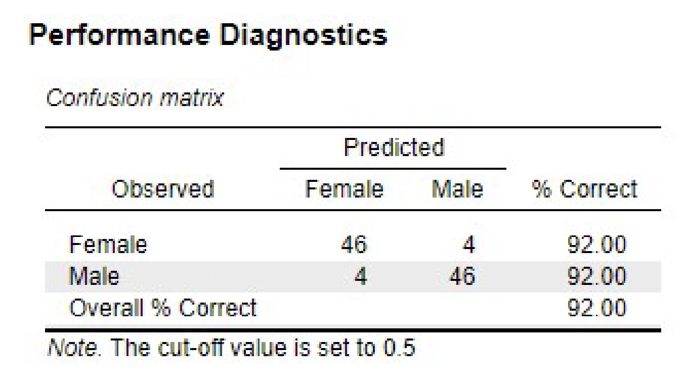
Confusion Matrix
A confusion matrix is a table used to evaluate the performance of a classification model. It summarizes the predicted classifications against percentage of correct predictions.
Predictive Accuracy
The accuracy of the logistic regression model can be evaluated using information criteria derived from the log-likelihood, such as the Akaike Information Criterion (AIC) and the Bayesian Information Criterion (BIC).
Akaike Information Criterion (AIC)
AIC is a measure used to compare the relative quality of statistical models for a given dataset. It balances model fit and complexity, penalizing models with more parameters to avoid overfitting.
Where is the number of parameters in the model and is the log-likelihood of the model.
Lower indicates better fit.
Bayesian Information Criterion (BIC)
BIC is similar to AIC but includes a stronger penalty for models with more parameters, especially as the sample size increases. It is used for model selection among a finite set of models.
Where is the number of observations, is the number of parameters in the model, and is the log-likelihood of the model.
Lower indicates better fit.
Self-Test
Simple Regression
- What are the key purposes of estimating a regression model?
- What are the key parameters of a regression model?
- How are the parameters of a regression model estimated?
- Why can it be helpful to center a predictor?
- How is a regression model evaluated statistically—both in terms of the overall model and in terms of the regression coefficients?
- What are key assumptions in simple linear regression—and how can you check whether the assumptions are fulfilled?
Multiple Regression
- Why can the regression coefficient for a predictor in a multiple regression differ from the regression coefficient in a simple regression?
- How can a multiple regression analysis be evaluated statistically (overall model fit, regression coefficients)?
- What is multicollinearity, when is it a problem, and how can one test for it?
- What aspects are relevant for a power analysis for multiple regression?
- How do you test whether a variable acts as a moderator in the relationship between two other variables?
- What are the steps of a mediation analysis?
- What is dummy coding and how it is used to include a categorical predictor in a regression model?
Logistic Regression
- In logistic regression, what does the linear combination of intercept and predictors predict?
- How are probability, odds, and log odds related to each other?
- How do you get from an estimated slope (i.e., regression coefficient) of a predictor to the odds ratio?
- How do you test whether an estimated regression coefficient differs significantly from zero?
- How can you assess the performance of a logistic regression model— with and without taking model complexity into account?
- What are key assumptions in logistic regression?
- How can you plan the sample size for a logistic regression analysis?