Multivariate Analysis — Reducing Data

Resources

• Slides: Factor Analysis, Cluster Analysis
• Exercises: Factor Analysis, Cluster Analysis

Factor Analysis determines similar groups of variables; Cluster Analysis determines similar groups of observations or objects.

Factor Analysis

Factor analysis is a statistical method used to identify underlying relationships, factors influencing covariation between observed variables. It reduces data dimensionality by grouping correlated variables into factors, which represent latent constructs.

Factor analysis refers both to the approach and a technique. Exploratory factor analysis is used to discover the underlying factor structure without prior hypotheses, while confirmatory factor analysis tests specific hypotheses about factor structures. Principle Component Analysis (PCA), however, provides a summary of a dataset’s correlational structure and allows for a mathematical transformation of the original variables into a smaller set of uncorrelated components, making it the standard technique for data reduction.

Latent Construct

A latent construct is an unobserved variable that influences observed variables. For example, “intelligence” is a latent construct that may influence test scores.

Suitability of Data for Factor Analysis

To conduct the factor analysis, the variables should be at least interval-scaled and approximately normally distributed. There should be multiple intercorrelations of .3 or higher among the variables to justify the analysis. In general, there should be at least 10 observations per variable and 4 variables per factor. Parameters become stable around 300 observations. With large communality, smaller samples may be sufficient.

Two tests can be used to assess the suitability of the data for factor analysis:

Bartlett's Test of Sphericity

Tests the null hypothesis that the correlation matrix is an identity matrix. A significant result (p < .05) indicates that there are sufficient correlations among variables to proceed with factor analysis.

Kaiser-Meyer-Olkin (KMO) Measure of Sampling Adequacy

Indicates the proportion of potentially common variance among variables. Values range from 0 to 1, with values above 0.6 generally considered acceptable for factor analysis.

$$\mathrm{KMO}=$$

\frac{ \sum_{j \neq k} \sum r_{jk}^2 }{ \sum_{j \neq k} \sum r_{jk}^2 ;+; \sum_{j \neq k} \sum p_{jk}^2 }

where $r_{jk}$ are the correlations between variables $j$ and $k$, and $p_{jk}$ is the correlation between $j$ and $k$ after all other variables have been partialled out.

Principle Component Analysis (PCA)

PCA is a technique of factor analysis that works with linear combinations of observed variables to create components that explain the maximum variance in the data. Each component is a weighted sum of the original variables, with weights determined by the eigenvectors of the correlation matrix. The first component explains the most variance, the second component explains the most of the remaining variance, and so on. Components are uncorrelated with each other.

Extraction of Factors

To determine the components to extract, we compute the eigenvalues and eigenvectors of the correlation matrix of the observed variables. The eigenvectors represent the directions of maximum variance (the components), and the eigenvalues indicate the amount of variance explained by each component.

The process was not further detailed mathematically here, but it’s solving the characteristic equation of the correlation matrix.

Determining Number of Factors to Keep

Several methods exist to determine the number of factors to retain in PCA:

• Kaiser Criterion: Retain factors with eigenvalues greater than 1.
• Scree Test: Plot the eigenvalues and look for an “elbow” point where the slope of the curve changes, indicating diminishing returns for additional factors. This approach is subjective.
• Parallel Analysis: Compare the eigenvalues from the actual data to those obtained from random data of the same size. Retain factors where the actual eigenvalue exceeds the random eigenvalue.

Eigenvalue Matrix

The eigenvalue matrix contains the eigenvalues associated with each principal component. Each eigenvalue represents the amount of variance in the data, across all variables, explained by its corresponding component. An eigenvalue greater than 1 indicates that the component explains more variance than a single observed variable.

$$L=V^{\prime }\cdot R\cdot V$$

where $L$ is the diagonal matrix of eigenvalues, $V$ is the matrix of eigenvectors (V’ transposed), and $R$ is the correlation matrix of the observed variables.

Eigenvalues

Eigenvalues are scalars associated with a linear transformation that indicate how much the transformation stretches or compresses vectors in a given direction. In the context of PCA, eigenvalues represent the amount of variance explained by each principal component.

Factor Loadings Matrix

The factor loading matrix shows the correlations between observed variables and the extracted factors. High loadings indicate that a variable is strongly associated with a factor. It’s determined by the eigenvalue matrix:

$$A=V\cdot \sqrt{L}$$

where $A$ is the factor loading matrix, $V$ is the matrix of eigenvectors, and $L$ is the diagonal matrix of eigenvalues.

• Factor Loading $a$: The correlation coefficient between an observed variable and a factor, indicating the strength and direction of their relationship.
• Communality $h^2$: The proportion of an observed variable’s variance explained by the common factors.
• Uniqueness: The proportion of an observed variable’s variance not explained by the common factors; the information lost when reducing dimensions. $1-\text{Communality}$

Factor Rotation

Variables may contribute to multiple factors, making interpretation difficult. Factor rotation helps with interpretation by maximizing high loadings and minimizing low loadings. When factors are rotated, the variables’ loadings on the factors are changed, but the overall fit of the model remains the same.

Geometric Representation

When representing factors as vectors, their correlation is the cosine of the angle between them. Orthogonal rotation keeps factors uncorrelated (90° angle), angles smaller than 90° indicate positive correlations, and angles larger than 90° indicate negative correlations. ((p. 21)) During rotation, the angles between factor axes change, and the factor loadings change accordingly. However, the lengths of the factor vectors (which determine communalities) and the total variance explained are preserved.

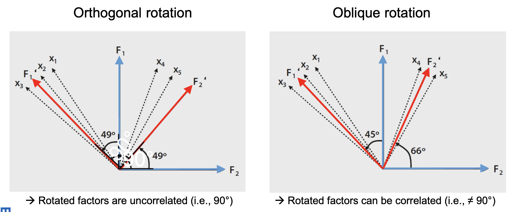
Orthogonal Rotation

Rotating orthogonally keeps factors uncorrelated. Choose this if the theory suggests that factors should be unrelated. Common methods include Varimax, Quartimax. Here, the axes of the factors are rotated while maintaining a 90° angle between them. Interpretation is based on structure loadings, which represent the total correlation of each factor with each variable.

• Varimax: Maximizes the variance of squared loadings across the variables within each factor.
• Quartimax: Maximizes the variance of squared loadings across factors for each variable.

Oblique Rotation

Oblique rotation allows the resulting factors to be correlated, reflecting real-world concepts that often relate. Common methods include Direct Oblimin, Promax. Here, the axes of the factors can take any angle relative to each other. Interpretation is based on pattern loadings, which represent the unique contribution of each factor to each variable.

• Oblimin: Minimizes the cross-loadings of variables on multiple factors.
• Promax recommended: Based on varimax rotation, but using exponentiated factor loadings to accentuate loading differences.

Factor Interpretation

After rotation, factors are interpreted based on the variables with high loadings. A common threshold is a loading of 0.4 or higher. Variables with high loadings on a factor are considered to contribute significantly to that factor, and a subjective judgement is made to label the factor based on the common theme among these variables.

Factor Scores

Factor scores represent each object’s position on the latent factors. They are computed as factor load-weighted variable combinations and can be used in further analyses to compare observations or examine relationships between factors and other variables.

Cluster Analysis

A statistical method used to group similar objects/observations into clusters based on their characteristics. The goal is to maximize similarity within clusters and minimize similarity between clusters. It can be seen as a complement to factor analysis, which reduces variables; cluster analysis reduces observations.

The goal is to find clusters such that:

• Internal Homogeneity: Objects within a cluster are as similar as possible.
• External Heterogeneity: Objects from different clusters are as dissimilar as possible.

1. Quantifying Similarity

Similarity between variables can be quantified through distance or correlation measures. The Euclidian distance is often a good starting point, though correlation-based similarity measures can be more appropriate when the focus is on patterns of variation rather than absolute values.

Euclidian Distance

The Euclidean distance between two points in a multi-dimensional space is calculated as:

$$d(p,q)=\sqrt{\sum _{j=1}^J|a_j-b_j{|}^2}$$

where $a$ and $b$ are two points in J-dimensional space.

Which simply measures the straight-line distance between two points; higher values indicate lower similarity.

Correlation-Based Similarity

Correlation-based similarity measures the degree to which two variables move together, even though they may be different in absolute space. The Pearson correlation coefficient is commonly used:

$$r_{a,b}=\frac{{\sum }_{j=1}^J(x_j^a-{\bar{x}}^a)\times (x_j^b-{\bar{x}}^b)}{\sqrt{{\sum }_{J=1}^J(x_j^a-{\bar{x}}^a{)}^2}\times \sqrt{{\sum }_{J=1}^J(x_j^b-{\bar{x}}^b{)}^2}}$$

where $x_j^a$ and $x_j^b$ are the values of variables a and b for observation j. Higher values indicate greater similarity.

2. Clustering Algorithms

Clusters are created step-by-step, often agglomeratively, but divisive methods also exist:

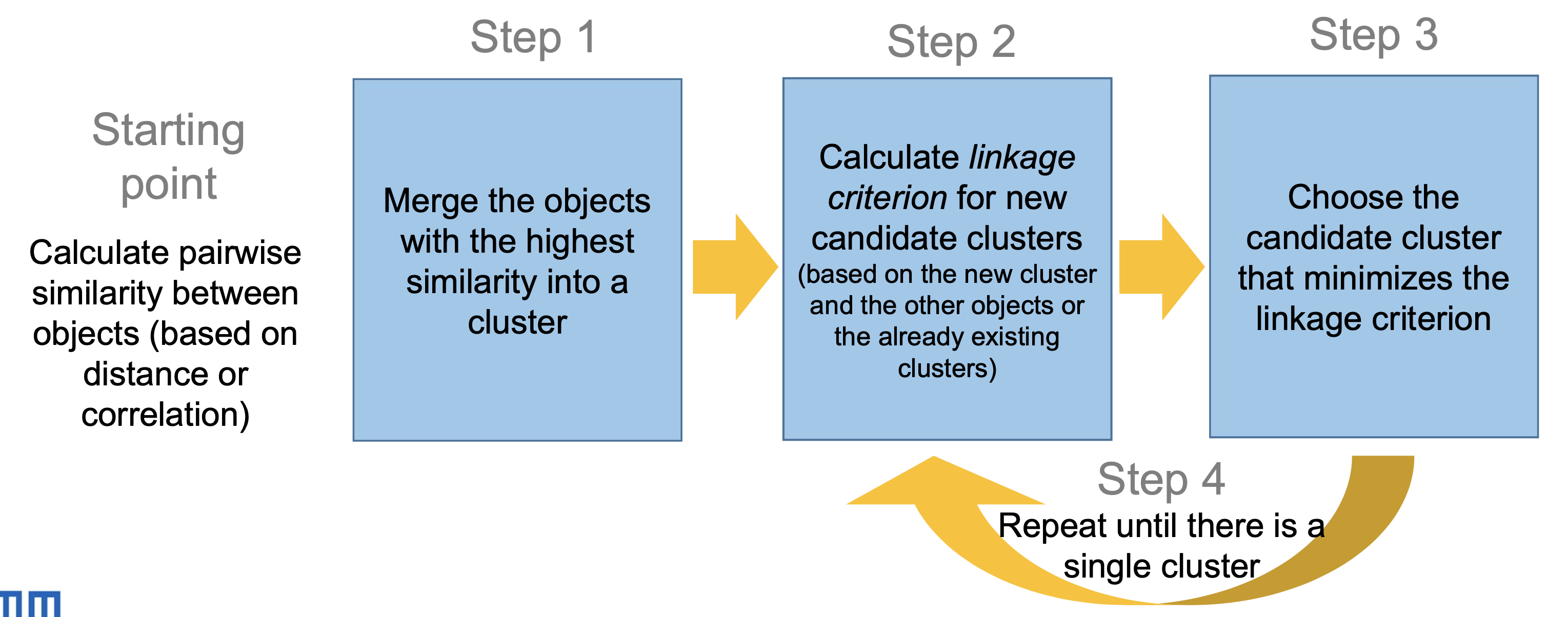
• Agglomerative Clustering: Start with each observation as its own cluster and iteratively merge the closest clusters until a stopping criterion is met.
• Divisive Clustering: Start with all observations in one cluster and iteratively split clusters until a stopping criterion is met.

In the agglomerative approach, objects with the highest similarity are merged first. Then, the similarity between clusters is recalculated using a linkage method and a new cluster is formed to minimize within-cluster variance. This is repeated until all objects are in a single cluster or a predefined number of clusters is reached.

Cluster Linkage

Linkage methods are criteria to decide which clusters to merge based on the distances between them. Common linkage methods include (visualizations on p. 23):

Single Linkage: Nearest Neighbor

Expresses the distance between clusters as the smallest distance between any pair of objects in the two clusters.

$$D(c_1,c_2)=\underset{x_1\in c_1,x_2\in c_2}{\min }(D(x_1,x_2))$$

Complete Linkage: Farthest Neighbor

Expresses the distance between clusters as the largest distance between any pair of objects in the two clusters.

$$D(c_1,c_2)=\underset{x_1\in c_1,x_2\in c_2}{\max }(D(x_1,x_2))$$

Ward's Method

This method can and should be used when Euclidean distance is the similarity measure. It describes the total distance of objects within a new candidate cluster.

It computes the centroid of two clusters, calculates the distance of each point to this centroid, and sums these distances to get the total within-cluster variance for the candidate. The centroid is the mean of all points in the candidate cluster.

$$T{D}_{c_1\cup c_2}=s_k^2=\sum _{i=1}^{I_k}\sum _{j=1}^J(x_{ijk}-{\bar{x}}_{jk}{)}^2$$

where ${\overline{x}}_{jk}$ is the centroid of cluster $k$ and $x_{ijk}$ are the observations in cluster $k$. $I_k$ is the number of observations in the new cluster, $J$ is the number of variables.

3. Optimizing the Number of Clusters

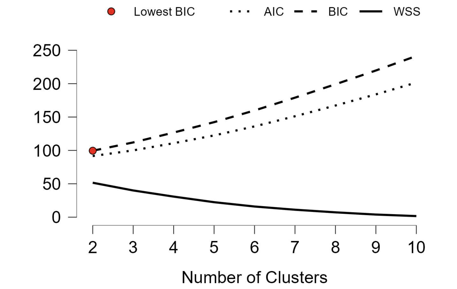
When using too many clusters, model complexity will outweigh model fit. Model fit can be measured using within-cluster sum of squares. The Akaike or Bayesian Information Critera trade off model fit against model complexity (number of clusters). The silhouette coefficient measures how well-separated clusters are while considering internal homogeneity for model fit.

It’s usually recommended to choose the solution with the lowest information criterion value (AIC or BIC), as it balances fit and complexity.

Within-Cluster Sum of Squares: WSS

The sum of the squares of the distances between objects and their cluster’s centroid. Lower values indicate more compact clusters, but model complexity and external heterogeneity are not considered. $WSS={\sum }_{k=1}^K{\sum }_{i=1}^{I_k}{\sum }_{j=1}^J(x_{ij}-{\bar{x}}_{jk}{)}^2$

Silhouette Coefficient

The silhouette coefficient measures how similar an object is to its own cluster compared to other clusters. It ranges from -1 to 1, with higher values indicating better-defined clusters where objects are more homogeneous within clusters and more distinct between clusters.

If most objects have a high positive silhouette value, the clustering configuration is appropriate. If many points have a negative silhouette value, the clustering configuration may have too many or too few clusters.

$s(i)=\frac{b(i)-a(i)}{\max \{a(i),b(i)\}}$

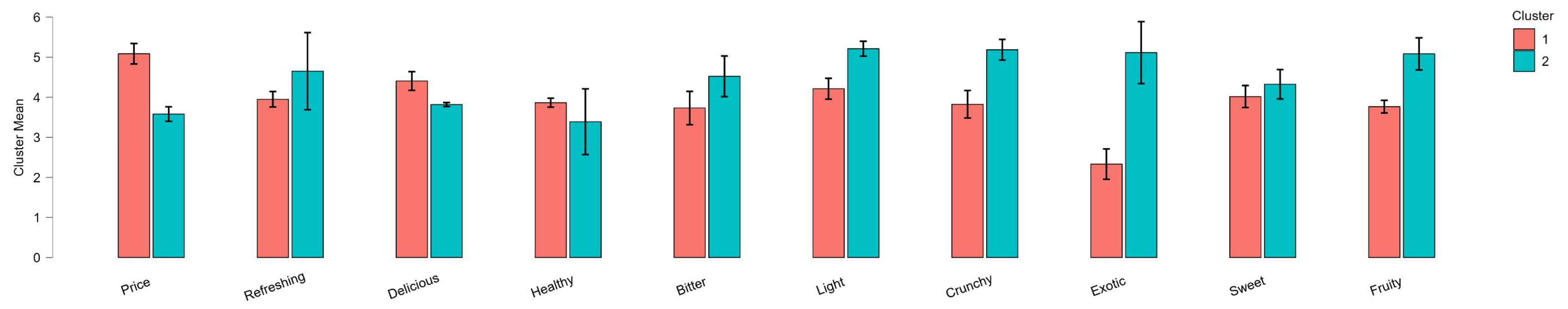
4. Interpreting Clusters

After determining the best clustering solutions, clusters may be interpreted in terms of their centroids or by examining the characteristics of objects within each cluster. One way is to visually inspect the dendogram. Alternatively, the average values of each variable within clusters can be compared to identify distinguishing features. (p. 31)

Visualizations

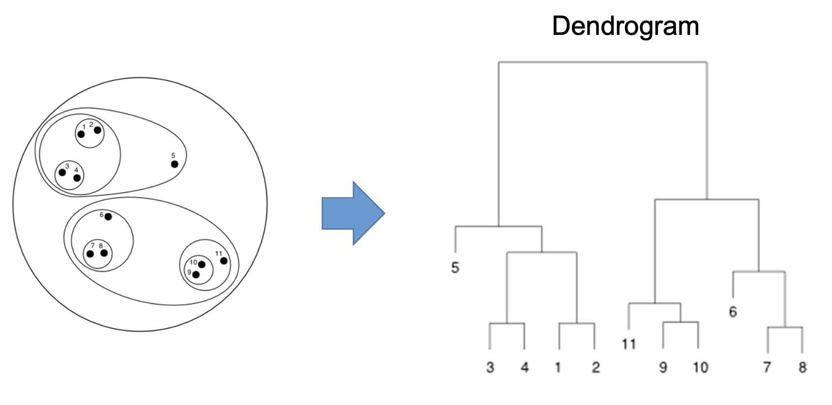
Dendrograms are tree-like diagrams that illustrate the arrangement of clusters formed by hierarchical clustering. The height at which two clusters are merged indicates the distance or dissimilarity between them. Dendograms are usually used over two-dimensional plots, which can be misleading due to dimensionality reduction.

Self-Test

Factor Analysis

• What are the goals of factor-analytic techniques?
• What do eigenvalues in a principle component analysis (PCA) represent?
• What is the key idea underlying the scree test? What is the purpose of parallel analysis?
• What are factor loadings? What is meant by uniqueness and how is it related to communality?
• Why is it usually useful to conduct a rotation of the extracted factor solution?
• What is the difference between orthogonal and oblique rotation?
• What are factor scores?
• What is measured with the Bartlett‘s test and the KMO test and what results of these tests are desirable?
• Give two rules of thumb when planning the sample size for a PCA