Inferential Statistics

Resources

• Slides Part 1, Slides Part 2
• Exercise Slides Part 1, Exercise Slides Part 2
• Recording Part 1, Recording Part 2

Sampling

Drawing inferences about a population based on data from a sample. (p. 7)

• Sampling Error: The difference between the characteristics of a sample and the characteristics of the population from which it was drawn. This error decreases as the sample size increases. (p. 7)

Examples for identifying sampling methods are available in the exercise slides. (p. 2)

Probability Sampling

Any person in the population has a specified probability of being included in the sample. This approach allows for generalization to the entire population. (p. 10)

Random Sampling

Each member of the population has an equal chance of being selected. This method minimizes selection bias and allows for generalization to the entire population.

Stratified Sampling

The population is divided into subgroups (strata) based on specific characteristics. Participants are then randomly sampled from these groups in proportion to their size in the population, ensuring representation on these traits.

Cluster Sampling

The population is divided into clusters (e.g., geographic areas), and a random sample of entire clusters is selected for the study. This method is cost-effective for large populations.

Non-Probability Sampling

Some members of the population are systematically excluded, leading to a non-representative sample. (p. 12)

Convenience Sampling

Samples are selected based on ease of access and availability. This method is prone to selection bias and limits generalizability.

Quota Sampling

The researcher sets quotas for specific subgroups to ensure representation, but selection within those subgroups is non-random (by convenience). This can introduce bias.

Snowball Sampling

Existing study subjects recruit future subjects from among their acquaintances. This is useful for hard-to-reach populations.

Purposive Sampling

Also known as judgmental sampling, participants are selected based on specific desirable characteristics, expertise, or qualities. This method is subjective and may not represent the population.

Sampling Distribution

The sampling distribution is the probability distribution of a statistic (e.g., the sample mean) obtained through a large number of samples drawn from a specific population. It provides insights into the variability and reliability of the statistic. This is compared to the population distribution to understand how well the sample represents the population.

Distribution of Sample Means

• The sampling distribution of the sample mean is the probability distribution of all possible sample means from a population.
• The mean of this distribution is equal to the population mean (${\mu }_{\bar{x}}=\mu$).
• Standard Error (SE): The standard deviation of the sampling distribution. It indicates the precision of the sample mean as an estimate of the population mean. (p. 15) $S{E}_{sample}=\frac{S{D}_{sample}}{\sqrt{n_{sample}}}$

Central Limit Theorem

• For a sufficiently large sample size (typically $n\ge 30$), the sampling distribution of the sample mean will be approximately normally distributed, regardless of the population’s distribution. (p. 16)

Statistical Hypothesis Testing

Fisherian Approach: Significance Testing

Focuses on the p-value to assess the evidence against a single hypothesis (the null hypothesis) without needing a pre-defined alternative hypothesis. (p. 22)

1. Define a null hypothesis ($H_0$) representing no effect or difference.
2. Define the expected probability distribution of results if $H_0$ were true.
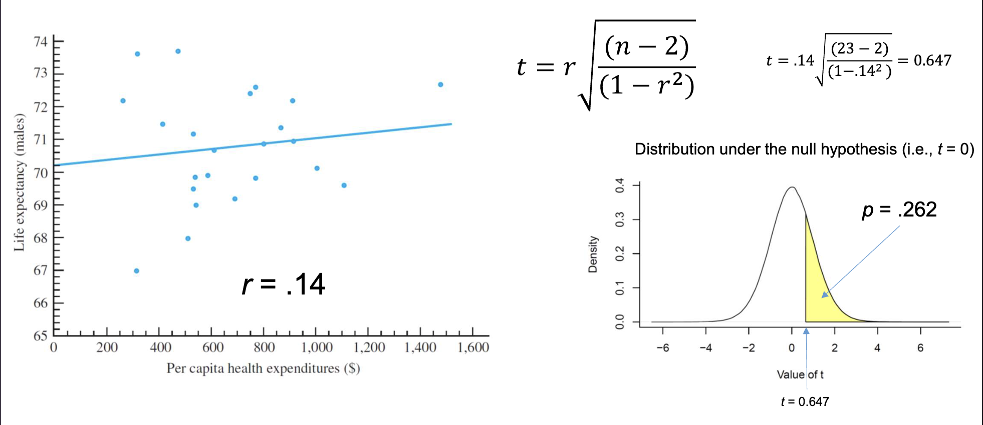
3. Significance Testing: Calculate the p-value, which is the probability of observing a result at least as extreme as the one obtained, assuming $H_0$ is true.

A small p-value suggests that the observed data is unusual under $H_0$. (p. 21)

Example: In the “lady tasting tea” experiment, the probability of her correctly identifying all 8 cups by chance ($H_0$) was p = .003, providing strong evidence against the null hypothesis. (p. 20)

Neyman-Pearson Approach: Hypothesis Testing

Focuses on making a decision between two competing hypotheses ($H_0$ and $H_1$) by controlling error rates. The goal is to minimize $\beta$ for a given $\alpha$. When $H_0$ is rejected, $H_1$ is accepted. (p. 27)

State of the World	Decision: Accept $H_0$	Decision: Accept $H_1$
$H_0$ is True	Correct Decision	Type I Error ($\alpha$)
$H_1$ is True	Type II Error ($\beta$)	Correct Decision (Power $1-\beta$)
[[Slides Lecture 4 Inferential I.pdf#page=26	(p. 26)]]

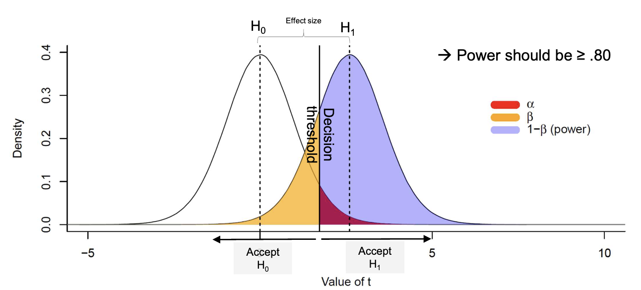
• Type I Error ($\alpha$): Rejecting $H_0$ when it is true (false positive). $\alpha$ is the significance level.
• Type II Error ($\beta$): Failing to reject $H_0$ when it is false (false negative).
• Power of a Test ($1-\beta$): The probability of correctly rejecting $H_0$ when it is false.
• Critical region: The range of values for which $H_0$ is rejected.

Null Hypothesis Significance Testing (NHST)

A modern hybrid approach combining elements from both Fisher and Neyman-Pearson. (p. 28)

• Effect Size: A standardized measure of the magnitude of an effect, representing the difference between the observed data and the null hypothesis $H_0$.

• Statistical Power ($1-\beta$): The probability of detecting an effect if it exists. Commonly set to .80.

1. Define the null hypothesis $H_0$.
2. Report the exact p-value, which is the probability of the observed data given $H_0$ is true ($p=P(\text{data}|H_0)$).
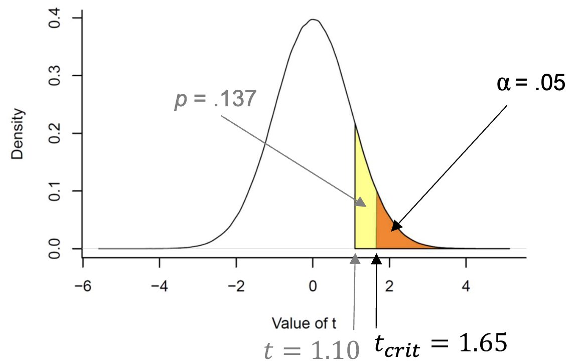
3. Compare the p-value to a predefined significance level ($\alpha$, usually .05 or .01).
4. If $p\le \alpha$, reject $H_0$; otherwise, fail to reject $H_0$.

Bayesian Statistics – Not relevant for exam (unless specified differently in last lecture)

An upcoming alternative. Focuses on updating the probability of a hypothesis based on observed data using Bayes’ theorem. It provides a more intuitive interpretation of evidence compared to NHST.

One-Tailed and Two-Tailed Tests

The choice depends on whether the research hypothesis is directional or non-directional. (p. 30)

One-Tailed Test

• Tests for an effect in a specific direction (e.g., greater than or less than).
• The entire significance level ($\alpha$) is placed in one tail of the sampling distribution.
• Used for directional hypotheses (e.g., $H_1:\mu >{\mu }_0$).

Two-Tailed Test

• Tests for an effect in any direction (i.e., not equal to).
• The significance level ($\alpha$) is split between both tails of the distribution ($\alpha /2$ in each tail).
• Used for non-directional hypotheses (e.g., $H_1:\mu \ne {\mu }_0$).

Statistical Power and Significance

Power

The probability of correctly rejecting a false null hypothesis ($1-\beta$). It is the likelihood of detecting an effect that is actually present.

Power is influenced by several factors: (p. 5)

• Effect Size: Larger effects are easier to detect, increasing power.
• Sample Size: Larger sample sizes provide more precise estimates, increasing power.
• Significance Level ($\alpha$): A higher $\alpha$ (e.g., .10 vs .05) increases power but also increases the risk of a Type I error.
• One-Tailed vs. Two-Tailed Tests: One-tailed tests have more power to detect an effect in the specified direction.
• Variability in Data: Lower data variability increases power.

An a-priori power analysis can be conducted before a study to determine the required sample size to achieve a desired level of power (e.g., .80). This can be done with software like G*Power. (p. 7)

Confidence Interval (CI)

• A range of values that likely contains the true population parameter with a certain level of confidence (e.g., 95% CI).
• Interpretation: If we were to repeat an experiment many times, 95% of the calculated confidence intervals would contain the true population parameter.

$CI=\bar{x}\pm Z_{\alpha /2}\times \frac{\sigma }{\sqrt{n}}$

t-Tests

Used to compare means between groups or conditions when the population standard deviation is unknown. This is applied to 1 Factor (independent variable) with 1 or 2 Levels (different groups).

t-Tests can be performed on independent samples (different groups), dependent samples (related measurement, e.g. same group), or single samples (to a specific value).

$$t=\frac{{\bar{X}}_1-{\bar{X}}_2}{{\hat{\sigma }}_{({\bar{X}}_1-{\bar{X}}_2)}}$$

which uses the estimated standard error of the difference between means:

$$\begin{array}{rlr}{\hat{\sigma }}_{({\bar{X}}_1-{\bar{X}}_2)}=\sqrt{\frac{{\hat{\sigma }}_{pooled}^2}{n_1}+\frac{{\hat{\sigma }}_{pooled}^2}{n_2}}& & {\hat{\sigma }}_{pooled}^2=\frac{{\hat{\sigma }}_1^2\ast (n_1-1)+{\hat{\sigma }}_2^2\ast (n_2-1)}{(n_1-1)+(n_2-1))}\end{array}$$

which is essentially a weighted average of the two sample variances.

t-Distribution

The distribution of a t-test statistic under the null hypothesis. It is shaped by degrees of freedom ($df$), which depend on the sample size(s). As $df$ increases, the t-distribution approaches the normal distribution. $df=n_1+n_2-2$

Effect Size

Cohen's d

A standardized measure of effect size that quantifies the difference between two means in terms of standard deviation units.

$$d=\frac{{\bar{X}}_1-{\bar{X}}_2}{\sqrt{{\hat{\sigma }}_{pooled}^2}}$$

$0.2$ is interpreted as a small effect, $0.5$ as medium, and $0.8$ as large.

ANOVA

Used to compare means across more than 2 levels (One-Way ANOVA) or multiple factors (Factorial ANOVA). It tests the null hypothesis that all group means are equal.

The F-statisic, the results of ANOVA (Analysis of Variance), is one-tailed. It is calculated as the ratio of variance between groups to variance within groups. If the groups differ meaningfully, the between‑group variance should be much larger than the within‑group variance — producing a large F‑statistic.

Sum of Squares

ANOVA starts by breaking total variability into meaningful parts using sum of squares (SS):

• SSTotal: variability of all observations around the grand mean
• SSBetween / SSFactor: variability explained by group differences
• SSInteraction (in factorial ANOVA): variability explained by combinations of factors
• SSWithin / SSResidual: leftover noise (differences within groups)

$SS=\sum (X_i-\bar{X}{)}^2$

Understanding SS helps interpret why the F‑statistic is large or small:

• High SSBetween → group means differ a lot
• High SSWithin → individuals within groups vary heavily (noisy data)
• SSInteraction → tells how much factors depend on each other (e.g., Age × Sex effects)

Mean Square

Each SS is divided by a degree of freedom to produce a mean square (MS): This converts raw variability into variances that can be compared fairly. $MS=\frac{SS}{df}$

F-Statistic

If groups truly differ, the numerator grows while the denominator stays roughly constant, resulting in a larger F-statistic for a given factor:

$F=\frac{M{S}_{\text{between}}}{M{S}_{\text{within}}}$

• Large F → strong evidence against the null hypothesis
• Small F → likely no meaningful group differences

F-Distribution

The distribution of the F-statistic under the null hypothesis.

It is defined by two sets of degrees of freedom:

• Numerator degrees of freedom ($d{f}_1$): associated with the between-group variability (e.g., number of groups - 1).
• Denominator degrees of freedom ($d{f}_2$): associated with the within-group variability (e.g., total sample size - number of groups).

To compute the p‑value, calculate the probability of observing an F‑statistic at least as large as the one calculated. F-statistics are always one-tailed.

Effect Size

Eta Squared ( ${\eta }^2$)

A measure of effect size for ANOVA that indicates the proportion of total variance in the dependent variable explained by the independent variable(s).

$${\eta }^2=\frac{S{S}_{Factor}}{S{S}_{Total}}$$

${\eta }^2$ overestimates the population value, especially for small $N$. 0.01 is interpreted as a small effect, 0.06 as medium, and 0.14 as large.

Omega Squared ( ${\omega }^2$)

A less biased measure of effect size for ANOVA that adjusts for the number of groups and sample size.

$${\omega }^2=\frac{S{S}_{Factor}-(d{f}_{Factor}\ast M{S}_{Error})}{S{S}_{Total}+M{S}_{Error}}$$

Chi-Square Test

Used to examine the association between two categorical variables. It tests the null hypothesis that the variables are independent. To perform the test, a contingency table is created to summarize the expected frequency counts for each combination of categories.

Then, the chi-square statistic (${\chi }^2$) is calculated by comparing the observed frequencies to the expected frequencies under the null hypothesis of independence:

${\chi }^2={\sum }_{i=1}^I{\sum }_{j=1}^J\frac{(n_{i,j}-e_{i,j}{)}^2}{e_{i,j}}$

• $n_{i,j}$ = observed frequency in cell (i,j)
• $e_{i,j}$ = expected frequency in cell (i,j) under $H_0$

A large chi-square statistic indicates a greater discrepancy between observed and expected frequencies, suggesting a potential association between the variables.

Chi-Square Distribution

The distribution of the chi-square statistic under the null hypothesis. It is defined by degrees of freedom ($df$), calculated as: $df=(I-1)(J-1)$ where $I$ is the number of rows and $J$ is the number of columns in the contingency table.

To compute the p‑value, calculate the probability of observing a chi-square statistic at least as large as the one calculated. Chi-square statistics are always one-tailed.

Effect Size

Cramér's V

This variable association measure can be used to determine the effect size of a Chi-Square Test. It’s further explained in Cramér’s V. $V=\sqrt{\frac{{\chi }^2}{n\ast \min (k-1,r-1)}}$ with $k$ = number of rows, $r$ = number of columns, and $n$ = total sample size.

An alternative method is the $\omega$ coefficient, which is less commonly used.